Test

The example code is in the file CPSstrainexample.tgz. First you must compile a program that is not in the Computer Programs in Seismology distribution: psac. This is a utility for plotting Sac files. First define a SHELL variable CPS that points to the location of the Computer Programs in Seismology package, such as

export CPS='/Users/rbh/PROGRAMS.310t/PROGRAMS.330/'

Then to execute this test case, do the following:

gunzip -f CPSstrainexample.tgz | tar xvf -
cd CPSstrain.example
make psac

DOIT
DOCLEANUP

The result of these computations will be the PNG files shown below: F14_5.png and F14_6.png.

the script DOIT invokes the scripts DOITWK, DOSTRAIN, DOPLTF14_5 and DOPTLF14_6 to do the following:

• DOIT: Top level script that invokes the other scripts, computes displacement and strain for different Cartesian system orientations, and converts the EPS files to PNG.
• DOITWK: Runs the programs hprep96 and hspec96strain to make synthetics for the CUS model at a distance of 200 km with source depth of 2.0 km and receiver depth of 0.0 km. The sample interval is 0.25s.
• DOSTRAIN: Create the time histories in Sac format for a source with duration of 2.0s. The source mechanism has strike of 0°, dip 90°, rake of 0° and Mw=2.6 (which corresponds to a moment of 1.0 x 10²⁰ dyne-cm. The observation azimuth is 45°
• DOPLT14_5: Compare the ground velocities and rotations at the receiver in terms of the cylindrical coordinate system.
• DOPLT14_6: Compare the u₁ and e₁₁ derived from the cylindrical values. This illustrates what might be seen if a single component horizontal sensor and a horizontal strainmeter has arbitrary orientations at the receiver point.
• DOCLEANUP: Remove all files created by the scripts. But keep the scripts and the PNG images.

Figures

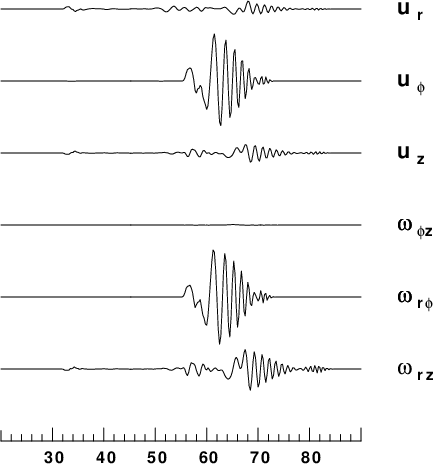
Comparison of ground velocities and rotations

Comparison of ground velocities (maximum value is 1.8 x 10^-7 m/s) and rotations (maximum value is 2.6 x 10^-11). As expected from plane wave simulations the u_φ velocity is similar to the ω_φ rotation. Also the u_z velocity is similar to the ω_rz rotation. Plane wave theory show that the ratios are proportional to the phase velocity.

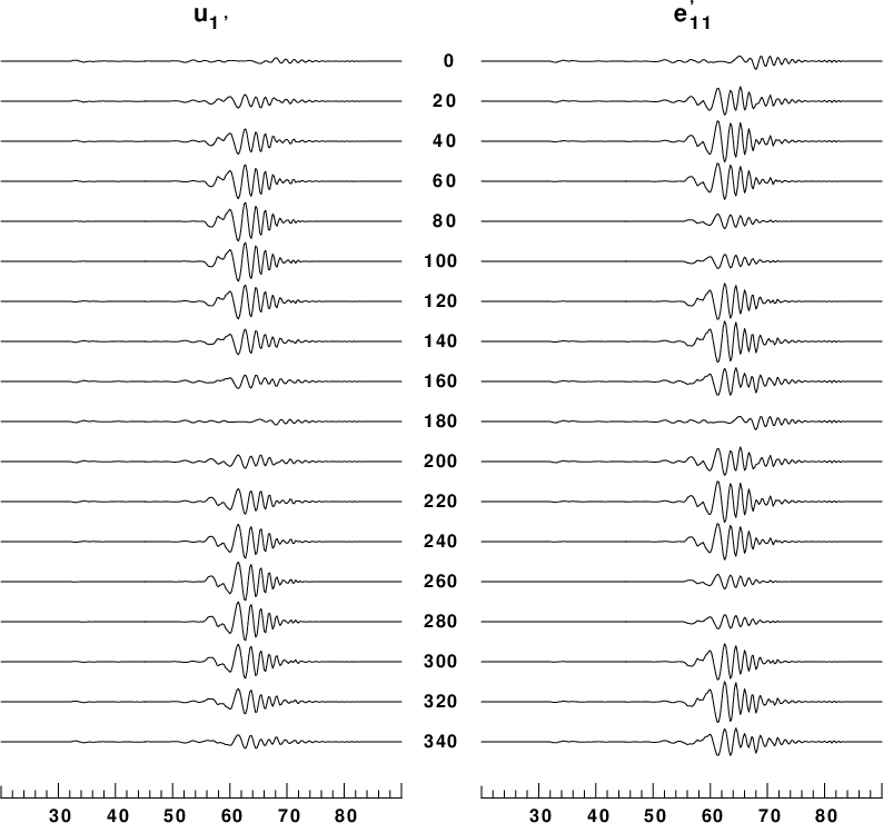
Comparison u1 and e11 as a function of local orientation

In this presentation, the velocity with maximum of 1.8 x 10 ^-7 m/s is in the left column and the strain with maximum value of 2.5 x 10^-11 is on the right column. The local coordinate system is rotated through angles of 0° to 340° with respect to the radial direction form the source. Since the signal is a mixture of Love and Rayleigh waves, the presentation shows the different radiation patterns of each.