Computer Programs in Seismology Tutorial

Introduction

This tutorial shows how to locate the epicenter of a seismic event using gsac, sac2eloc and elocate.

Data preparation

The file event.tgz contains the Sac waveform files used in this tutorial. Unpack the files with the command

gunzip -c event.tgz | tar xvf -

This will create the subdirectory DAT which contains the waveform files. You can check to see that the files have the station coordinates properly installed with the command

gsac
GSAC> rh *
GSAC> lh stla stlo stel
GSAC> q

Note that the gsac invokes the code and that the GSAC> are the interactive prompts of the program.

Arrival picking using gsac

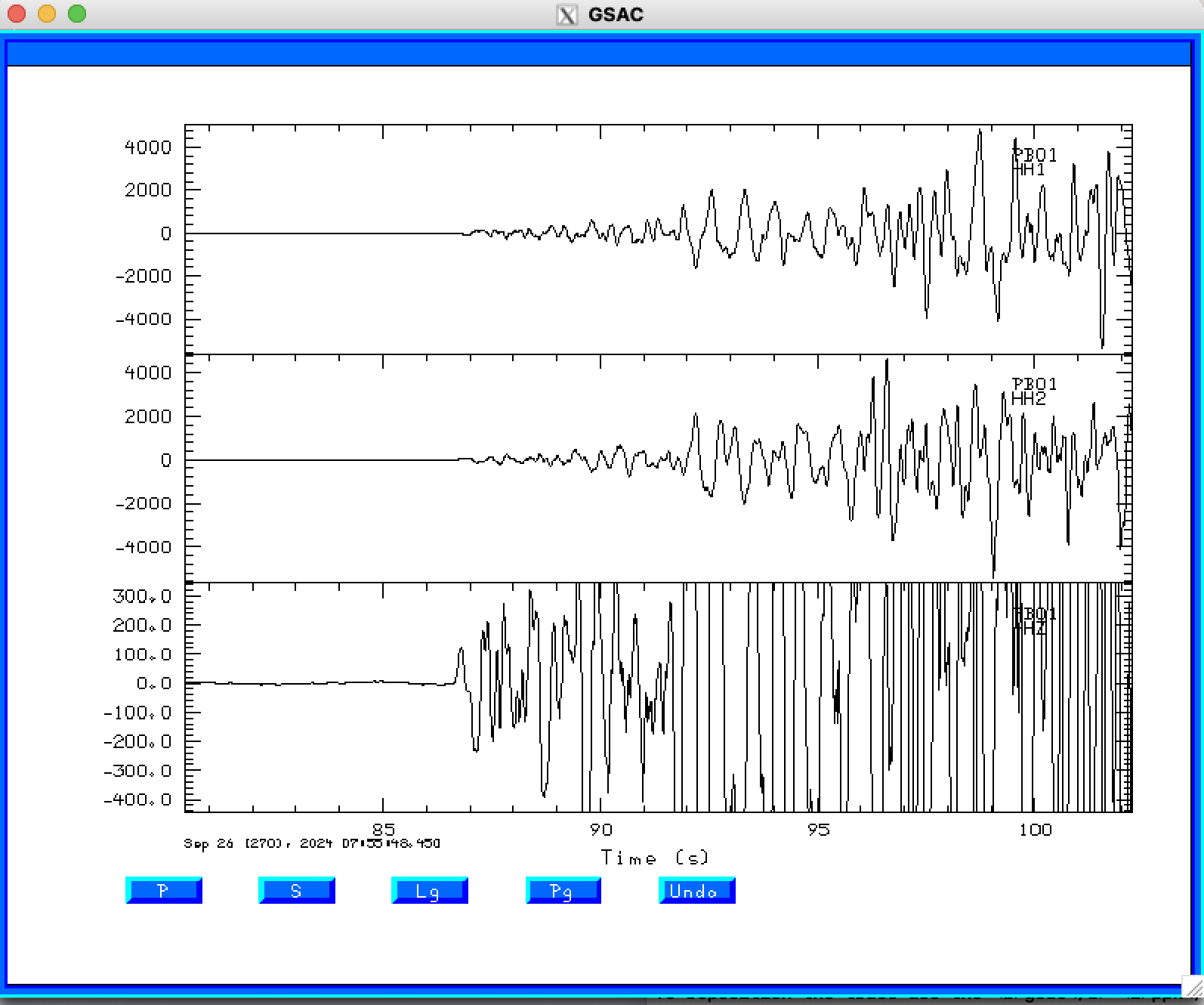
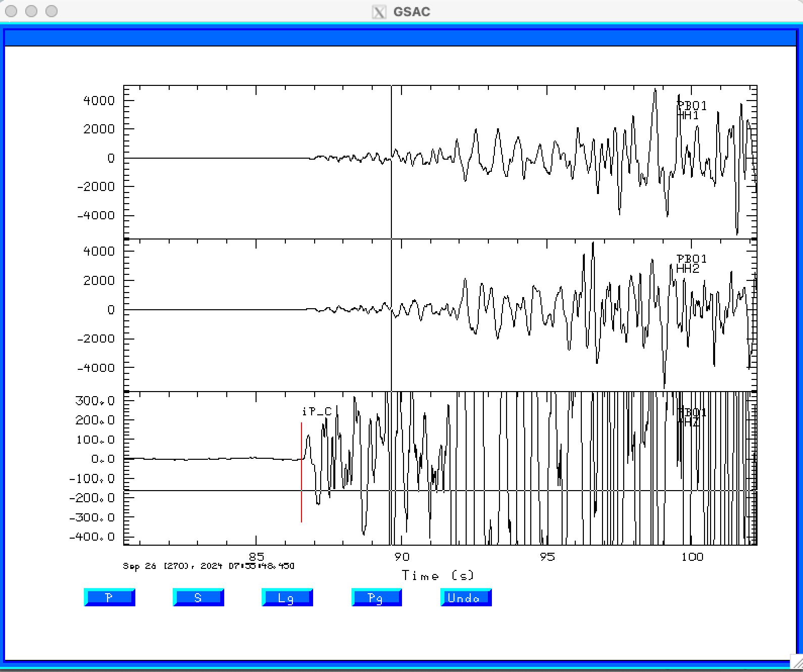
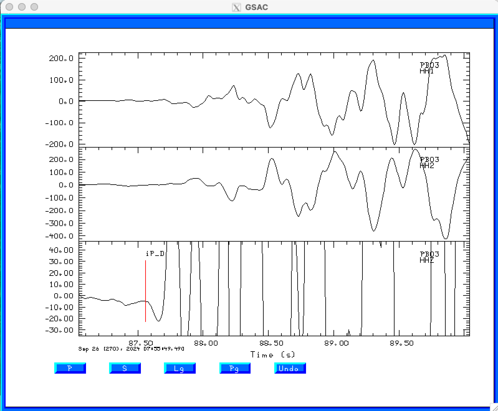
gsac is used to pick the arrival times which are then saved in the header of each sac file. One can use the plotpk or the shorthand ppk to enter the interactive mode and then use 'P' or 'S' commands to time a phase. While this is can be done, gsac has a GUI to make picking easier. One enters the command ppk REG to pick arrivals for local and regional events or ppk TEL for teleseisms. The GUI permits the use to set arrival weights, polarities, and phase name. The example here uses the GUI.

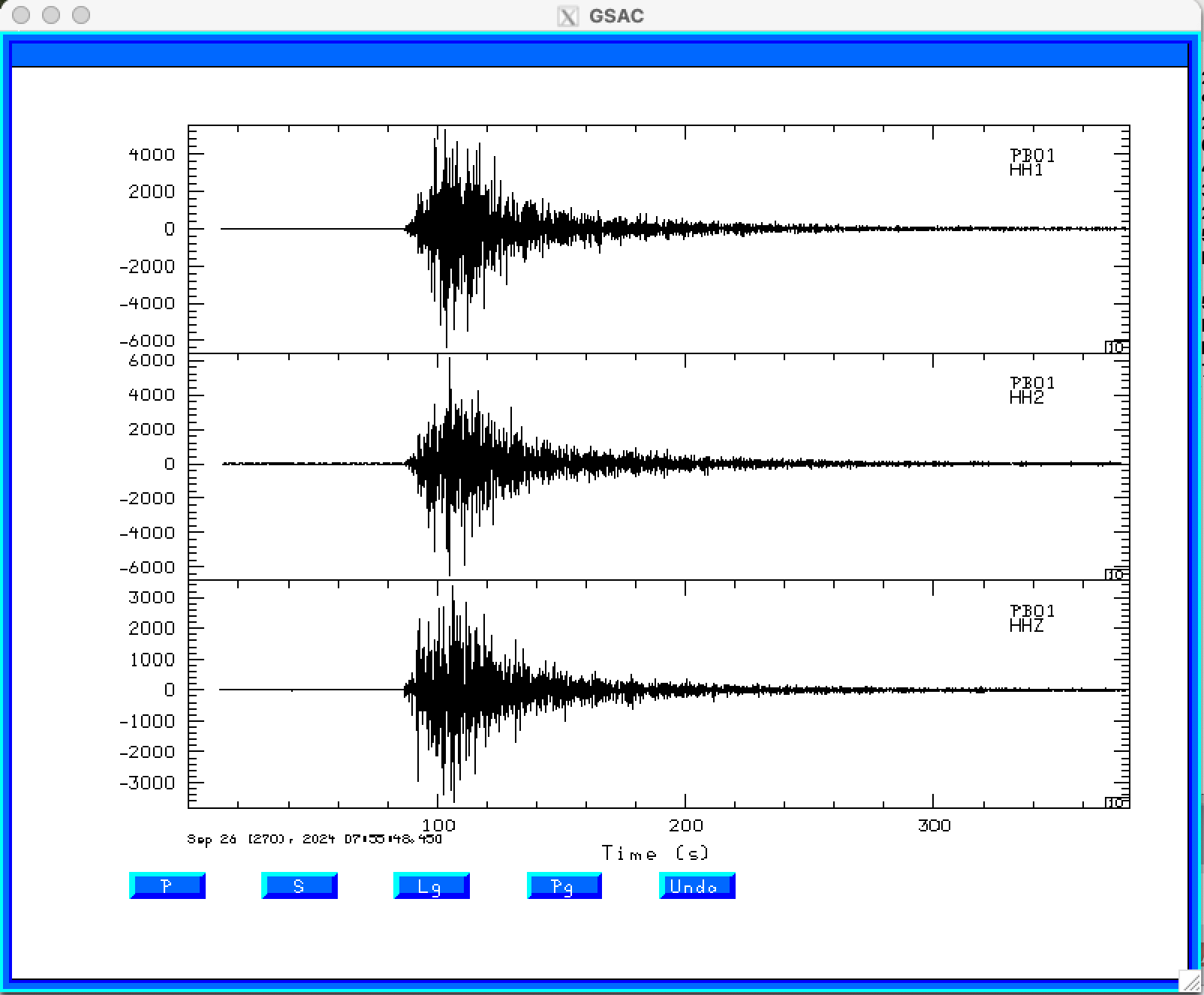
cd DAT
gsac
GSAC> r *
GSAC> ppk regional
   ...      [the GUI appears]
   ...      [when done picking, save the picks in the header of each sac file]
GSAC> wh
GSAC> q

For the data set the following shows the commands and interactive session:

cd DAT
gsac
GSAC> r *
GSAC> rtr
GSAC> hp c 1 n 2
GSAC> lp c 3 n 2   [For regional events this is a good frequency band for picking]
GSAC> qdp 10       [To make the display faster, only display every 10th point.
                    This is permissible since we just did a low pass ]
GSAC> ppk perplot 3 regional
                   [Use the regional picking GUI and display three traces at 
                    a time since the stations have 3 components of motion]

The result of this sequence is the window


The cursor is an arrow outside of the traces and a crosshair within the trace subwindows. To reposition the trace use the gsac ppk options [GSAC> help ppk]. The "x x" will permit a selection of part of the trace, the "*" "." or the mouse wheel will change the amplitude of the trace, and a "+" or "-" will center the trace on the cursor point and zoom in or out, respectively. The first traces, e.g., for station PB01, do not seem to have a strong S. After entering "x" and moving the cursor and entering the second "x" and using the mouse wheel on the Z component, we get Figure 2:


Now the P arrival is obvious. To pick the arrival click on the "P" button, move the cursor to the trace and click on the aligned arrival. The "i" and "e" buttons appear - select "i" is this is a sharp arrival and "e" if it is emergent. This choice affects the arrival weight. After this select the polarity. "C" for a strong compression, usually up/positive on the vertical, "+" for a weak compression, "D" for a strong dilatation/down, "-" for a weak down, and "X" for an indeterminate first motions. The pick is now displayed. If you do not like it, hit the "Undo" button.


If you are finished with this trace, enter "n" to go to the next trace. If you want to back up to a previous trace, enter "b". For the next trace I picked the S on the HH1 channel and zoomed in on the P arrival on the HHZ trace and then increased the amplitude to see the small initial downward motions.


When you are done picking "q" from the interactive picking, or after looking a all traces, you will be returned tot he command prompt. Here you will save the picks using the "wh" / "writeheader" command. Do not use the "w" / "write" command since the original traces will be overwritten by the filtered traces that you used.

GSAC> wh
GSAC> q

sac2eloc

To locate the event, we need to place the arrival picks and other information into the file elocate.dat.

To avoid cluttering the directory containing the sac files, we will work in the directory above. thus enter the command

sac2eloc DAT/*SAC  #[since the sac files ended as .SAC]

The result is the file elocate.dat.

elocate

This program is described in Chapter 5of the  gsac tutorial that is the file cps330g.pdf in the directory PROGRAMS.330/DOC/GSAC.pdf of the source distribution.

elocate has some built in velocity models but Chapter 5 discusses the format of the VEL.MOD file so that a user defined velocity model can be used.

Since elocate is discussed in cps330g.pdf, the following will show the commands used to locate the event. The processing will be in the batch, e.g., non-interactive mode. The user is encouraged to run the program interactively to appreciate how the choice of the velocity model and initial source depth can affect the solution, since event location is a non-linear  problem.

If you first execute elocate you will be presented with the velocity models in the file VEL.MOD. The WUS model is identified as "7". So a batch run using the WUS model would be

elocate -VELMOD       #[Creates the file VEL.MOD in the directory.]
elocate -M 7 -D 10 -BATCH > elocate.txt   
#[Use model 7, an initial depth of 10 km and batch (automatic run.}

The output of this run is in the file elocate.txt. The first part of this file shows the data which includes the station, weight, arrival time,. phase and polarity, and station latitude, longitude and elevation [Note: elocate does not use elevation corrections]. The results of the iterations is next which gives latitude, longitude, depth, origin time, and RMS error. Obviously there is some observation that causes a big residual. After the maximum number of iterations is achieved or the solution converges, the fit to each phase is given. Here the P arrival at PB17 has a large residual, and that trace should be reexamined. Note that this was weighted 0.00 in the inversion because of the large residual. The final part, reproduced here is the solution:

 Error Ellipse  X=   1.7949 km  Y= 2.7735 km  Theta = 348.0448 deg (azimuth of X axis)

 RMS Error        :               1.694              sec
 Travel_Time_Table:          WUS     
 Latitude         :             31.5325 +-    0.0166 N         1.8476 km
 Longitude        :           -104.1199 +-    0.0290 E         2.7387 km
 Depth            :               12.90 +-      2.68 km
 Epoch Time       :      1727337407.380 +-      0.62 sec
 Event Time       :  20240926075647.380 +-      0.62 sec
 Event (OCAL)     :  2024 09 26 07 56 47 380
 HYPO71 Quality   :                  DB
 Gap              :                 130              deg
 
    ch evla    31.5325 evlo  -104.1199 evdp      12.90
    ch ocal   2024 09 26 07 56 47 380
 
    ch o gmt   2024 270  07 56 47 380

The last three line are gsac commands if you wish to place the location information in the sac files, e.g.,

gsac
GSAC> rh *SAC
GSAC>   ch evla    31.5325 evlo  -104.1199 evdp      12.90
GSAC>   ch ocal   2024 09 26 07 56 47 380
GSAC> wh
GSAC> q

If the CMPINC and CMPAZ fields are set in the header, you are ready to rotate the three component traces to make Z, R and T traces.

Several output files are created: fmplot.tmp, assoc.tmp, origin.tmp. orger.tmp and elocate.sum. They contain information from the elocate.txt listing. The fmplot.tmp can be use with the program fmplot to plot the first motions. In this example, there is a proposed focal mechanism (solid curves) that is compared to the observations. The commands are

#!/bin/sh

elocate -VELMOD
elocate -M 7 -BATCH -D 10 > elocate.txt

# compare the first motion to this solution
STK=320
DIP=40
RAKE=-80

fmplot -S $STK -D $DIP -R $RAKE -F fmplot.tmp -tp
plotnps -BGFILL -F7 -W10 -EPS -K < FMPLOT.PLT > t.eps
# Use ImageMagick to convert EPS to PNG
convert -trim t.eps slufm.png

The result is ithe file slufm.png

The fit is not good, mostly because the initial P amplitudes read were very small. The elocate solution gives the azimuth to the station and also the takeoff angle of the P way to the station. This angle is measured from the downward vertical. If the depth changes, or if a different model is used, the takeoff angle will change.

Discussion

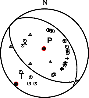I sometimes use elocate in the processing of regional moment tensors which the time shift between the observed and predicted waveforms indicates a mislocation. I also run this code then the moment tensor is not what was expected given its location. In this case I compare the moment tensor nodal planes and P (pressure) and T (tension) axes to P-wave first motions. Given perfect data sets and the correct regional velocity model, the moment tensor mechanism and depth should agree with observed p-wave first motions and hypocenter. This is the ideal validation of a solution.

If you have an independent solution, with the event coordinates set in the SAC file headers, the traces can be rotated. Further theoretical arrival times for a model can be entered into the header given the distance and source depth in the header. Often I find that the S arrival is sharper on the T (transverse component), and thus read it from that component.