
 USGS/SLU Moment Tensor Solution
 ENS  2021/08/13 11:57:35:0  35.88  -84.90   1.0 3.5 Tennessee

 Stations used:
   CO.CASEE CO.HODGE CO.PAULI ET.CPCT IM.TKL IU.WCI IU.WVT
   N4.R49A N4.R50A N4.S51A N4.T47A N4.T50A N4.U49A N4.V48A
   N4.V53A N4.V55A N4.W50A N4.W52A N4.X48A N4.X51A N4.Y52A
   NM.BLO NM.USIN US.GOGA US.LRAL US.TZTN

 Filtering commands used:
   cut o DIST/3.3 -40 o DIST/3.3 +50
   rtr
   taper w 0.1
   hp c 0.03 n 3
   lp c 0.10 n 3

 Best Fitting Double Couple
  Mo = 8.32e+21 dyne-cm
  Mw = 3.88
  Z  = 8 km
  Plane   Strike  Dip  Rake
   NP1       41    60   -87
   NP2      215    30   -95
  Principal Axes:
   Axis    Value   Plunge  Azimuth
    T   8.32e+21     15     129
    N   0.00e+00      2     219
    P  -8.32e+21     75     318

 Moment Tensor: (dyne-cm)
    Component   Value
       Mxx     2.70e+21
       Mxy    -3.50e+21
       Mxz    -2.89e+21
       Myy     4.47e+21
       Myz     3.03e+21
       Mzz    -7.18e+21


                     ##############
                 ############---------#
              ##########------------------
             ########---------------------#
           ########-----------------------###
          #######------------------------#####
         #######-------------------------######
        #######-------------------------########
        ######----------   -------------########
       ######----------- P ------------##########
       ######-----------   -----------###########
       #####-------------------------############
       #####-----------------------##############
        ####----------------------##############
        ####--------------------################
         ###------------------#################
          ###---------------############   ###
           ##-------------############## T ##
             #--------##################
              ############################
                 ######################
                     ##############


 Global CMT Convention Moment Tensor:
      R          T          P
 -7.18e+21  -2.89e+21  -3.03e+21
 -2.89e+21   2.70e+21   3.50e+21
 -3.03e+21   3.50e+21   4.47e+21


Details of the solution is found at

http://www.eas.slu.edu/eqc/eqc_mt/MECH.NA/20210813115735/index.html
|
      STK = 215
      DIP = 30
     RAKE = -95
       MW = 3.88
       HS = 8.0
The NDK file is 20210813115735.ndk The waveform inversion is preferred.
The following compares this source inversion to others
 USGS/SLU Moment Tensor Solution
 ENS  2021/08/13 11:57:35:0  35.88  -84.90   1.0 3.5 Tennessee

 Stations used:
   CO.CASEE CO.HODGE CO.PAULI ET.CPCT IM.TKL IU.WCI IU.WVT
   N4.R49A N4.R50A N4.S51A N4.T47A N4.T50A N4.U49A N4.V48A
   N4.V53A N4.V55A N4.W50A N4.W52A N4.X48A N4.X51A N4.Y52A
   NM.BLO NM.USIN US.GOGA US.LRAL US.TZTN

 Filtering commands used:
   cut o DIST/3.3 -40 o DIST/3.3 +50
   rtr
   taper w 0.1
   hp c 0.03 n 3
   lp c 0.10 n 3

 Best Fitting Double Couple
  Mo = 8.32e+21 dyne-cm
  Mw = 3.88
  Z  = 8 km
  Plane   Strike  Dip  Rake
   NP1       41    60   -87
   NP2      215    30   -95
  Principal Axes:
   Axis    Value   Plunge  Azimuth
    T   8.32e+21     15     129
    N   0.00e+00      2     219
    P  -8.32e+21     75     318

 Moment Tensor: (dyne-cm)
    Component   Value
       Mxx     2.70e+21
       Mxy    -3.50e+21
       Mxz    -2.89e+21
       Myy     4.47e+21
       Myz     3.03e+21
       Mzz    -7.18e+21


                     ##############
                 ############---------#
              ##########------------------
             ########---------------------#
           ########-----------------------###
          #######------------------------#####
         #######-------------------------######
        #######-------------------------########
        ######----------   -------------########
       ######----------- P ------------##########
       ######-----------   -----------###########
       #####-------------------------############
       #####-----------------------##############
        ####----------------------##############
        ####--------------------################
         ###------------------#################
          ###---------------############   ###
           ##-------------############## T ##
             #--------##################
              ############################
                 ######################
                     ##############


 Global CMT Convention Moment Tensor:
      R          T          P
 -7.18e+21  -2.89e+21  -3.03e+21
 -2.89e+21   2.70e+21   3.50e+21
 -3.03e+21   3.50e+21   4.47e+21


Details of the solution is found at

http://www.eas.slu.edu/eqc/eqc_mt/MECH.NA/20210813115735/index.html
|
 Moment (dyne-cm)   7.34E+21   dyne-cm
 Magnitude (Mw)    3.84
 Depth   4.0 km

 Principal Axes:
   Axis    Value   Plunge  Azimuth
    T   7.34E+21     48.    159.
    N  -9.30E+17      4.     65.
    P  -7.34E+21     42.    331.
 Moment Tensor: (dyne-cm) Aki-Richards               Lune parameters
    Component   Value
       Mxx   -2.01E+20                                beta:   90.00
       Mxy    6.17E+20                                gamma:  -0.01
       Mxz   -6.62E+21
       Myy   -5.30E+20
       Myz    3.04E+21
       Mzz    7.31E+20
 Global CMT Convention Moment Tensor: (dyne-cm)
         R         T         F
  R  7.31E+20 -6.62E+21 -3.04E+21
  T -6.62E+21 -2.01E+20 -6.17E+20
  F -3.04E+21 -6.17E+20 -5.30E+20


                    --------------                         :
                ---------------------#                   :---:
             ---------------------------#              ::. ..::
            ------------------------------            :--------:
          ----------   --------------------#         :: .  . .  :
         ----------- P ---------------------#        :  .  .  .  :
        ------------   -----------------------      :------------::
       ---------------------------------######-    ::  .   .  .   :
       -----------------------------##########-    :   .   .   .  :
      -------------------------################-   :---------------:
      ---------------------####################-   :   .   .   .   :
      -----------------########################-   :=======#=======:
      -------------############################-   :   .   .   .   :
       ---------##############################-    :   .   .   .   :
       -----##################################-    :---------------:
        -####################   #############-     :   .   .   .  :
         #################### T ############-      ::  .   .  .   :
          ###################   ###########-        :------------::
            #############################-           :  .  .  .  :
             ##########################--            :: .  . .  :
                #####################-                :--------:
                    #############-                     ::. ..::
                                                         :---:
                                                           :
|
 Moment (dyne-cm)   1.06E+22   dyne-cm
 Magnitude (Mw)    3.95
 Depth   8.0 km

 Principal Axes:
   Axis    Value   Plunge  Azimuth
    T   6.58E+21      0.    203.
    N   5.62E+21      7.    113.
    P  -1.22E+22     83.    297.
 Moment Tensor: (dyne-cm) Aki-Richards               Lune parameters
    Component   Value
       Mxx    6.38E+21                                beta:   89.93
       Mxy    4.54E+20                                gamma:  27.39
       Mxz   -9.76E+20
       Myy    5.55E+21
       Myz    1.94E+21
       Mzz   -1.19E+22
 Global CMT Convention Moment Tensor: (dyne-cm)
         R         T         F
  R -1.19E+22 -9.76E+20 -1.94E+21
  T -9.76E+20  6.38E+21 -4.54E+20
  F -1.94E+21 -4.54E+20  5.55E+21


                    ##############                         :
                ######################                   :---:
             ############################              ::. ..::
            ###########-----##############            :--------:
          ########---------------###########         :: .  . .  :
         #######-------------------##########        :  .  .  .  :
        ######-----------------------#########      :------------::
       ######-------------------------#########    ::  .   .  .   :
       #####---------------------------########    :   .   .   .  :
      ######------------   ------------#########   :---------------:
      ######------------ P ------------#########   :   .   .   .   :
      ######------------   ------------#########   :==============#:
      ######---------------------------#########   :   .   .   .   :
       ######-------------------------#########    :   .   .   .   :
       #######-----------------------##########    :---------------:
        ########--------------------##########     :   .   .   .  :
         #########----------------###########      ::  .   .  .   :
          ############--------##############        :------------::
            ##############################           :  .  .  .  :
             ############################            :: .  . .  :
                ###   ################                :--------:
                    T ############                     ::. ..::
                                                         :---:
                                                           :
|
 Moment (dyne-cm)   1.43E+22   dyne-cm
 Magnitude (Mw)    4.04
 Depth   5.0 km

 Principal Axes:
   Axis    Value   Plunge  Azimuth
    T  -3.98E+21     14.    106.
    N  -4.78E+21      2.    196.
    P  -1.92E+22     76.    293.
 Moment Tensor: (dyne-cm) Aki-Richards               Lune parameters
    Component   Value
       Mxx   -4.85E+21                                beta:  143.11
       Mxy    1.11E+20                                gamma:  27.33
       Mxz   -1.37E+21
       Myy   -4.80E+21
       Myz    3.31E+21
       Mzz   -1.83E+22
 Global CMT Convention Moment Tensor: (dyne-cm)
         R         T         F
  R -1.83E+22 -1.37E+21 -3.31E+21
  T -1.37E+21 -4.85E+21 -1.11E+20
  F -3.31E+21 -1.11E+20 -4.80E+21


                    --------------                         :
                ----------------------                   :---:
             ----------------------------              ::. ..::
            ------------------------------            :--------:
          ----------------------------------         :: .  . .  :
         ------------------------------------        :  .  .  .  :
        --------------------------------------      :------------::
       ----------------------------------------    ::  .   .  .   :
       ----------------------------------------    :   .   .   .  :
      -----------------   ----------------------   :---------------:
      ----------------- P ----------------------   :   .   .   .   :
      -----------------   ----------------------   :===============:
      -------------------------------------   --   :   .   .   .   :
       ------------------------------------ T -    :   .   .   .   :
       ------------------------------------   -    :---------------:
        --------------------------------------     :   .   .   .  :
         ------------------------------------      ::  .   .  .   :
          ----------------------------------        :------------::
            ------------------------------           :  .  .  .  :
             ----------------------------            :: .  . .  #
                ----------------------                :--------:
                    --------------                     ::. ..::
                                                         :---:
                                                           :
|
 Moment (dyne-cm)   1.36E+22   dyne-cm
 Magnitude (Mw)    4.02
 Depth   6.0 km

 Principal Axes:
   Axis    Value   Plunge  Azimuth
    T  -3.39E+21      3.    114.
    N  -5.86E+21     20.     23.
    P  -1.79E+22     69.    213.
 Moment Tensor: (dyne-cm) Aki-Richards               Lune parameters
    Component   Value
       Mxx   -6.50E+21                                beta:  144.95
       Mxy   -1.60E+21                                gamma:  20.89
       Mxz    3.29E+21
       Myy   -4.25E+21
       Myz    2.27E+21
       Mzz   -1.64E+22
 Global CMT Convention Moment Tensor: (dyne-cm)
         R         T         F
  R -1.64E+22  3.29E+21 -2.27E+21
  T  3.29E+21 -6.50E+21  1.60E+21
  F -2.27E+21  1.60E+21 -4.25E+21


                    --------------                         :
                ----------------------                   :---:
             ----------------------------              ::. ..::
            ------------------------------            :--------:
          ----------------------------------         :: .  . .  :
         ------------------------------------        :  .  .  .  :
        --------------------------------------      :------------::
       ----------------------------------------    ::  .   .  .   :
       ----------------------------------------    :   .   .   .  :
      ------------------------------------------   :---------------:
      ------------------------------------------   :   .   .   .   :
      ------------------------------------------   :===============:
      -----------------   ----------------------   :   .   .   .   :
       ---------------- P ---------------------    :   .   .   .   :
       ----------------   ------------------       :---------------:
        ------------------------------------ T     :   .   .   .  :
         -----------------------------------       ::  .   .  .   :
          ----------------------------------        :------------::
            ------------------------------           :  .  .  .  :
             ----------------------------            :: .  . .# :
                ----------------------                :--------:
                    --------------                     ::. ..::
                                                         :---:
                                                           :
|
 Moment (dyne-cm)   9.83E+21   dyne-cm
 Magnitude (Mw)    3.93
 Depth   8.0 km

 Principal Axes:
   Axis    Value   Plunge  Azimuth
    T   7.44E+21      4.    109.
    N   3.70E+21     13.     18.
    P  -1.11E+22     76.    216.
 Moment Tensor: (dyne-cm) Aki-Richards               Lune parameters
    Component   Value
       Mxx    3.55E+21                                beta:   90.00
       Mxy   -1.53E+21                                gamma:  19.04
       Mxz    2.66E+21
       Myy    6.74E+21
       Myz    2.27E+21
       Mzz   -1.03E+22
 Global CMT Convention Moment Tensor: (dyne-cm)
         R         T         F
  R -1.03E+22  2.66E+21 -2.27E+21
  T  2.66E+21  3.55E+21  1.53E+21
  F -2.27E+21  1.53E+21  6.74E+21


                    ##############                         :
                ######################                   :---:
             ############################              ::. ..::
            ##############################            :--------:
          ##################################         :: .  . .  :
         ###########------------#############        :  .  .  .  :
        ##########----------------############      :------------::
       #########--------------------###########    ::  .   .  .   :
       ########----------------------##########    :   .   .   .  :
      ########-----------------------###########   :---------------:
      #######-------------------------##########   :   .   .   .   :
      #######----------   ------------##########   :============#==:
      ######----------- P ------------##########   :   .   .   .   :
       #####-----------   ------------######       :   .   .   .   :
       ######------------------------####### T     :---------------:
        #####-----------------------########       :   .   .   .  :
         #####----------------------#########      ::  .   .  .   :
          #####-------------------##########        :------------::
            #####---------------##########           :  .  .  .  :
             ######-----------###########            :: .  . .  :
                ######################                :--------:
                    ##############                     ::. ..::
                                                         :---:
                                                           :
|
|
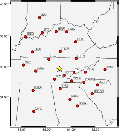
The focal mechanism was determined using broadband seismic waveforms. The location of the event and the and stations used for the waveform inversion are shown in the next figure.
|
|
|
The program wvfgrd96 was used with good traces observed at short distance to determine the focal mechanism, depth and seismic moment. This technique requires a high quality signal and well determined velocity model for the Green functions. To the extent that these are the quality data, this type of mechanism should be preferred over the radiation pattern technique which requires the separate step of defining the pressure and tension quadrants and the correct strike.
The observed and predicted traces are filtered using the following gsac commands:
cut o DIST/3.3 -40 o DIST/3.3 +50
rtr
taper w 0.1
hp c 0.03 n 3
lp c 0.10 n 3
The results of this grid search from 0.5 to 19 km depth are as follow:
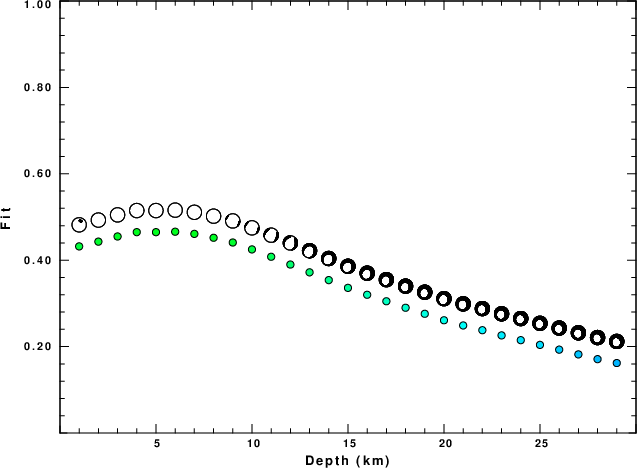
           DEPTH  STK   DIP  RAKE   MW    FIT
WVFGRD96    1.0   225    15    90   3.94 0.3003
WVFGRD96    2.0    50     5    90   3.94 0.3374
WVFGRD96    3.0    40     5    80   3.88 0.3516
WVFGRD96    4.0    10     5    35   3.84 0.3530
WVFGRD96    5.0   295     5   -40   3.82 0.3503
WVFGRD96    6.0   250    10   -85   3.82 0.3507
WVFGRD96    7.0   230    20   -95   3.84 0.3495
WVFGRD96    8.0   215    30   -95   3.88 0.3530
WVFGRD96    9.0    35    55   -90   3.90 0.3518
WVFGRD96   10.0    35    60   -90   3.90 0.3336
WVFGRD96   11.0    30    55   -95   3.91 0.3256
WVFGRD96   12.0    30    55   -95   3.91 0.3148
WVFGRD96   13.0   220    35   -85   3.90 0.3013
WVFGRD96   14.0   220    35   -85   3.90 0.2862
WVFGRD96   15.0   220    40   -80   3.90 0.2706
WVFGRD96   16.0   220    40   -80   3.90 0.2559
WVFGRD96   17.0   225    45   -80   3.90 0.2426
WVFGRD96   18.0   225    50   -80   3.90 0.2304
WVFGRD96   19.0   225    50   -80   3.91 0.2180
WVFGRD96   20.0   225    50   -80   3.93 0.2004
WVFGRD96   21.0   225    50   -80   3.93 0.1904
WVFGRD96   22.0   225    50   -80   3.93 0.1804
WVFGRD96   23.0   220    30   -80   3.94 0.1716
WVFGRD96   24.0   220    30   -80   3.94 0.1640
WVFGRD96   25.0   220    30   -80   3.94 0.1565
WVFGRD96   26.0   220    30   -80   3.95 0.1493
WVFGRD96   27.0   220    30   -80   3.95 0.1423
WVFGRD96   28.0   220    30   -80   3.95 0.1358
WVFGRD96   29.0   220    30   -80   3.96 0.1296
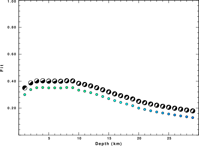
The best solution is
WVFGRD96 8.0 215 30 -95 3.88 0.3530
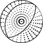
The mechanism correspond to the best fit is
|
|
|
The best fit as a function of depth is given in the following figure:
|
|
|
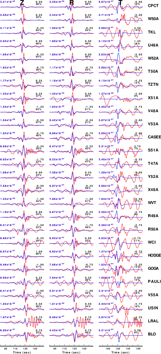
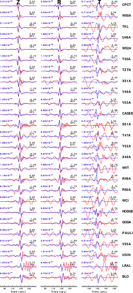
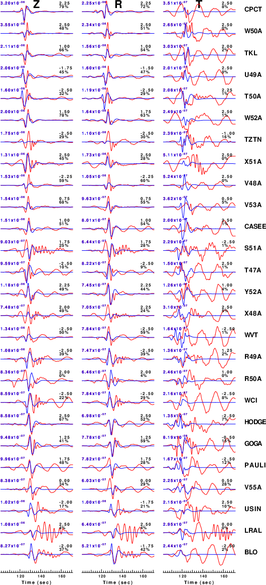
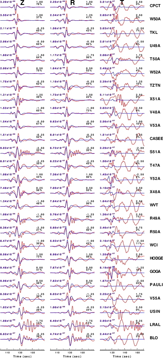
The comparison of the observed and predicted waveforms is given in the next figure. The red traces are the observed and the blue are the predicted. Each observed-predicted component is plotted to the same scale and peak amplitudes are indicated by the numbers to the left of each trace. A pair of numbers is given in black at the right of each predicted traces. The upper number it the time shift required for maximum correlation between the observed and predicted traces. This time shift is required because the synthetics are not computed at exactly the same distance as the observed and because the velocity model used in the predictions may not be perfect. A positive time shift indicates that the prediction is too fast and should be delayed to match the observed trace (shift to the right in this figure). A negative value indicates that the prediction is too slow. The lower number gives the percentage of variance reduction to characterize the individual goodness of fit (100% indicates a perfect fit).
The bandpass filter used in the processing and for the display was
cut o DIST/3.3 -40 o DIST/3.3 +50
rtr
taper w 0.1
hp c 0.03 n 3
lp c 0.10 n 3

|
|
|
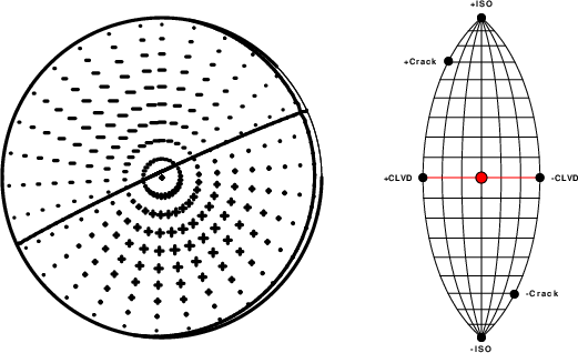
|
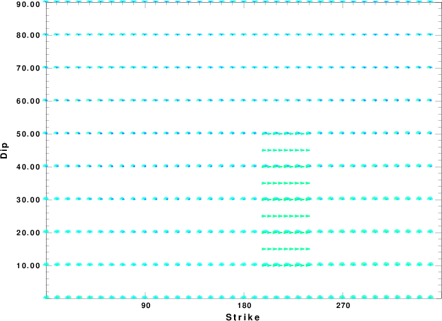
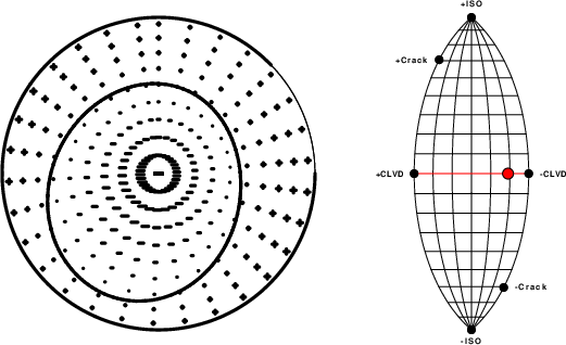
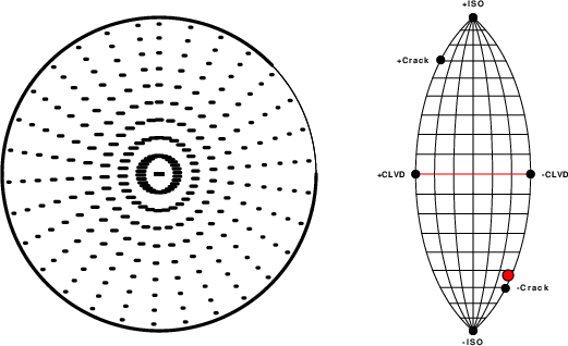
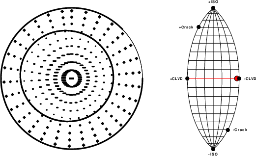
| Focal mechanism sensitivity at the preferred depth. The red color indicates a very good fit to thewavefroms. Each solution is plotted as a vector at a given value of strike and dip with the angle of the vector representing the rake angle, measured, with respect to the upward vertical (N) in the figure. |
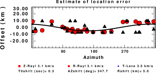
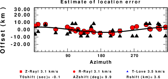
A check on the assumed source location is possible by looking at the time shifts between the observed and predicted traces. The time shifts for waveform matching arise for several reasons:
Time_shift = A + B cos Azimuth + C Sin Azimuth
The time shifts for this inversion lead to the next figure:

The derived shift in origin time and epicentral coordinates are given at the bottom of the figure.
The focal mechanism was determined using broadband seismic waveforms. The location of the event and the and stations used for the waveform inversion are shown in the next figure.

|
|
|
The program wvfmtd96 was used with good traces observed at short distance to determine the focal mechanism, depth and seismic moment. This technique requires a high quality signal and well determined velocity model for the Green functions. To the extent that these are the quality data, this type of mechanism should be preferred over the radiation pattern technique which requires the separate step of defining the pressure and tension quadrants and the correct strike.
The observed and predicted traces are filtered using the following gsac commands:
cut o DIST/3.3 -40 o DIST/3.3 +50
rtr
taper w 0.1
hp c 0.03 n 3
lp c 0.10 n 3
The results of this grid search over depth are as follow:
MT Program H(km)                    Mw                           Fit                              Mxx(dyne-cm)    Myy           Mxy            Mxz            Myz            Mzz
WVFMTD961    1.0  112.   77.   88.   4.02     0.362 0.168E-06     0.407     0.602 0.989E-07  62.4 -0.3319895E+22 -0.4711893E+22  0.2337869E+21  0.1063262E+23  0.3905504E+22  0.8031787E+22
WVFMTD961    2.0  110.   72.   89.   3.97     0.285 0.177E-06     0.314     0.534 0.106E-06  78.6 -0.3546755E+22 -0.4938356E+22  0.4039407E+21  0.7953777E+22  0.2709646E+22  0.8485112E+22
WVFMTD961    3.0  112.   78.   97.   3.92     0.274 0.179E-06     0.307     0.523 0.107E-06  76.7 -0.2531185E+22 -0.3171754E+22  0.1541076E+22  0.7157846E+22  0.3935299E+22  0.5702939E+22
WVFMTD961    4.0  313.   71. -101.   3.86     0.207 0.187E-06     0.235     0.456 0.112E-06  58.5  0.1762375E+22  0.4005270E+22  0.5367612E+21  0.5102345E+22  0.3090363E+22 -0.5767646E+22
WVFMTD961    5.0  338.   56. -105.   3.93     0.270 0.179E-06     0.310     0.519 0.107E-06  77.6  0.3557526E+22  0.6513655E+22  0.1078676E+20  0.3731448E+22  0.2235274E+22 -0.1007118E+23
WVFMTD961    6.0  360.   52. -106.   3.94     0.331 0.172E-06     0.380     0.575 0.101E-06  74.9  0.3892329E+22  0.6908235E+22 -0.9472948E+21  0.2946250E+22  0.2332079E+22 -0.1080056E+23
WVFMTD961    7.0    5.   51. -106.   3.93     0.364 0.167E-06     0.414     0.603 0.984E-07  71.8  0.3822746E+22  0.6764081E+22 -0.1254516E+22  0.2732953E+22  0.2293528E+22 -0.1058683E+23
WVFMTD961    8.0    7.   51. -107.   3.93     0.374 0.166E-06     0.425     0.612 0.974E-07  66.5  0.3547503E+22  0.6743559E+22 -0.1525908E+22  0.2660663E+22  0.2270451E+22 -0.1029106E+23
WVFMTD961    9.0    8.   49. -107.   3.92     0.373 0.166E-06     0.422     0.611 0.977E-07  64.8  0.3433997E+22  0.6788356E+22 -0.1558295E+22  0.2744943E+22  0.1783633E+22 -0.1022235E+23
WVFMTD961   10.0   12.   48. -108.   3.95     0.365 0.167E-06     0.410     0.604 0.988E-07  71.9  0.4270352E+22  0.6823130E+22 -0.1651534E+22  0.3013550E+22  0.2010756E+22 -0.1109348E+23
WVFMTD961   11.0   13.   48. -108.   3.94     0.358 0.168E-06     0.400     0.598 0.995E-07  71.7  0.4182432E+22  0.6621923E+22 -0.1669159E+22  0.2965003E+22  0.2072089E+22 -0.1080436E+23
WVFMTD961   12.0   13.   49. -108.   3.94     0.347 0.170E-06     0.387     0.589 0.101E-06  72.4  0.4133767E+22  0.6463232E+22 -0.1631316E+22  0.2931837E+22  0.2110035E+22 -0.1059700E+23
WVFMTD961   13.0   12.   49. -108.   3.93     0.334 0.171E-06     0.371     0.578 0.102E-06  73.7  0.4110089E+22  0.6349517E+22 -0.1545114E+22  0.2902847E+22  0.2161274E+22 -0.1045961E+23
WVFMTD961   14.0   12.   49. -109.   3.93     0.319 0.173E-06     0.353     0.565 0.103E-06  76.7  0.4129878E+22  0.6121386E+22 -0.1474122E+22  0.3077418E+22  0.2220998E+22 -0.1025126E+23
WVFMTD961   15.0   12.   49. -109.   3.93     0.305 0.175E-06     0.337     0.552 0.105E-06  78.3  0.4223258E+22  0.6051908E+22 -0.1397619E+22  0.2996347E+22  0.2273997E+22 -0.1027517E+23
WVFMTD961   16.0   11.   49. -109.   3.93     0.291 0.177E-06     0.320     0.539 0.106E-06  79.7  0.4206896E+22  0.6067470E+22 -0.1316206E+22  0.3088233E+22  0.2288248E+22 -0.1027437E+23
WVFMTD961   17.0    3.   51. -107.   3.93     0.277 0.178E-06     0.305     0.526 0.107E-06  78.1  0.3952786E+22  0.6449878E+22 -0.1081212E+22  0.3089237E+22  0.2353325E+22 -0.1040266E+23
WVFMTD961   18.0    1.   51. -107.   3.94     0.264 0.180E-06     0.291     0.514 0.108E-06  77.6  0.3939501E+22  0.6647686E+22 -0.9944994E+21  0.3132404E+22  0.2315125E+22 -0.1058719E+23
WVFMTD961   19.0    0.   52. -107.   3.94     0.252 0.182E-06     0.276     0.502 0.109E-06  77.6  0.4030284E+22  0.6805277E+22 -0.9563083E+21  0.3144489E+22  0.2342851E+22 -0.1083556E+23
WVFMTD961   20.0  358.   52. -106.   3.97     0.238 0.183E-06     0.261     0.488 0.111E-06  79.9  0.4535439E+22  0.7392234E+22 -0.9195459E+21  0.3522346E+22  0.2715694E+22 -0.1192767E+23
WVFMTD961   21.0  357.   52. -104.   3.98     0.227 0.184E-06     0.250     0.477 0.111E-06  82.2  0.4929441E+22  0.7459270E+22 -0.6875909E+21  0.3124538E+22  0.2569650E+22 -0.1238871E+23
WVFMTD961   22.0  357.   53. -103.   3.98     0.217 0.186E-06     0.238     0.465 0.112E-06  81.6  0.5000453E+22  0.7578449E+22 -0.6761278E+21  0.3064898E+22  0.2783754E+22 -0.1257890E+23
WVFMTD961   23.0  357.   53. -103.   3.98     0.206 0.187E-06     0.226     0.454 0.113E-06  82.2  0.5134203E+22  0.7641737E+22 -0.6762390E+21  0.3051191E+22  0.2883592E+22 -0.1277594E+23
WVFMTD961   24.0  356.   53. -102.   3.99     0.195 0.188E-06     0.215     0.442 0.114E-06  83.2  0.5347837E+22  0.7760174E+22 -0.5674828E+21  0.2972454E+22  0.2876322E+22 -0.1310801E+23
WVFMTD961   25.0  355.   52. -102.   3.99     0.185 0.189E-06     0.204     0.430 0.115E-06  82.3  0.5336987E+22  0.8009540E+22 -0.5135833E+21  0.3091200E+22  0.2613456E+22 -0.1334653E+23
WVFMTD961   26.0  349.   53. -101.   4.00     0.175 0.191E-06     0.193     0.418 0.115E-06  83.2  0.5502241E+22  0.8078016E+22 -0.2492438E+21  0.3113257E+22  0.2649643E+22 -0.1358026E+23
WVFMTD961   27.0  344.   54.  -99.   4.00     0.165 0.192E-06     0.182     0.406 0.116E-06  81.9  0.5605465E+22  0.8215537E+22  0.8663718E+20  0.3090834E+22  0.2741319E+22 -0.1382100E+23
WVFMTD961   28.0  342.   54. -100.   4.01     0.155 0.193E-06     0.171     0.395 0.117E-06  83.0  0.5635581E+22  0.8225153E+22  0.7325070E+20  0.3446980E+22  0.2606917E+22 -0.1386073E+23
WVFMTD961   29.0  342.   54. -101.   4.01     0.147 0.194E-06     0.162     0.384 0.117E-06  82.4  0.5569865E+22  0.8376288E+22  0.3891990E+20  0.3678209E+22  0.2623384E+22 -0.1394615E+23
The best solution is
WVFMTD961 8.0 7. 51. -107. 3.93 0.374 0.166E-06 0.425 0.612 0.974E-07 66.5 0.3547503E+22 0.6743559E+22 -0.1525908E+22 0.2660663E+22 0.2270451E+22 -0.1029106E+23
The complete moment tensor decomposition using the program mtdinfo is given in the text file MTDinfo.txt. (Jost, M. L., and R. B. Herrmann (1989). A student's guide to and review of moment tensors, Seism. Res. Letters 60, 37-57. SRL_60_2_37-57.pdf.
The P-wave first motion mechanism corresponding to the best fit is
|
|
|
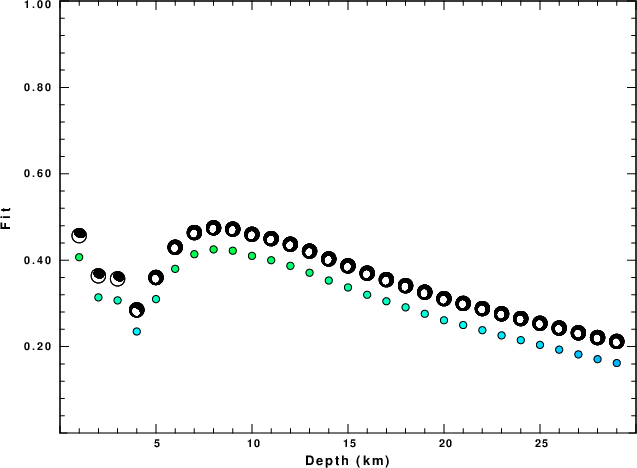
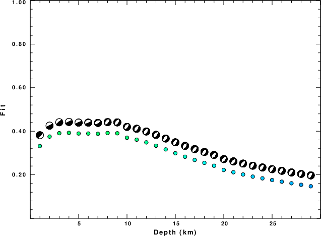
The best fit as a function of depth is given in the following figure:
|
|
|
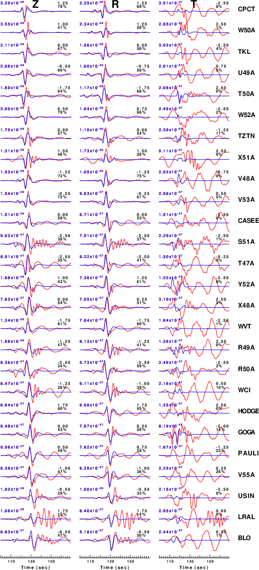
The comparison of the observed and predicted waveforms is given in the next figure. The red traces are the observed and the blue are the predicted. Each observed-predicted component is plotted to the same scale and peak amplitudes are indicated by the numbers to the left of each trace. A pair of numbers is given in black at the right of each predicted traces. The upper number it the time shift required for maximum correlation between the observed and predicted traces. This time shift is required because the synthetics are not computed at exactly the same distance as the observed and because the velocity model used in the predictions may not be perfect. A positive time shift indicates that the prediction is too fast and should be delayed to match the observed trace (shift to the right in this figure). A negative value indicates that the prediction is too slow. The lower number gives the percentage of variance reduction to characterize the individual goodness of fit (100% indicates a perfect fit).
The bandpass filter used in the processing and for the display was
cut o DIST/3.3 -40 o DIST/3.3 +50
rtr
taper w 0.1
hp c 0.03 n 3
lp c 0.10 n 3
|
|
|
A check on the assumed source location is possible by looking at the time shifts between the observed and predicted traces. The time shifts for waveform matching arise for several reasons:
Time_shift = A + B cos Azimuth + C Sin Azimuth
The time shifts for this inversion lead to the next figure:

The derived shift in origin time and epicentral coordinates are given at the bottom of the figure.
The focal mechanism was determined using broadband seismic waveforms. The location of the event and the and stations used for the waveform inversion are shown in the next figure.

|
|
|
The program wvfmt96 was used with good traces observed at short distance to determine the focal mechanism, depth and seismic moment. This technique requires a high quality signal and well determined velocity model for the Green functions. To the extent that these are the quality data, this type of mechanism should be preferred over the radiation pattern technique which requires the separate step of defining the pressure and tension quadrants and the correct strike.
The observed and predicted traces are filtered using the following gsac commands:
cut o DIST/3.3 -40 o DIST/3.3 +50
rtr
taper w 0.1
hp c 0.03 n 3
lp c 0.10 n 3
The results of this grid search over depth are as follow:
MT Program H(km)                    Mw                           Fit                              Mxx(dyne-cm)    Myy           Mxy            Mxz            Myz            Mzz
WVFMT961    1.0  292.   85.  -88.   4.07     0.385 0.165E-06     0.432     0.621 0.968E-07   6.7 -0.8151812E+22 -0.9438619E+22  0.2258521E+21  0.9685494E+22  0.4045636E+22 -0.1173597E+23
WVFMT961    2.0  295.   74.  -88.   4.08     0.396 0.163E-06     0.443     0.630 0.960E-07  50.5 -0.9177980E+22 -0.1001612E+23  0.1203198E+21  0.5426428E+22  0.2753143E+22 -0.1691299E+23
WVFMT961    3.0  294.   68.  -87.   4.08     0.406 0.162E-06     0.455     0.638 0.949E-07  76.4 -0.8887105E+22 -0.9185225E+22 -0.1564870E+21  0.4190254E+22  0.2242015E+22 -0.1838509E+23
WVFMT961    4.0  238.   52.  -64.   4.07     0.415 0.161E-06     0.465     0.644 0.941E-07  96.5 -0.8356662E+22 -0.7580230E+22 -0.8221667E+21  0.3553262E+22  0.2102310E+22 -0.1847023E+23
WVFMT961    5.0    5.   52. -117.   4.04     0.415 0.160E-06     0.465     0.645 0.940E-07  85.2 -0.7443625E+22 -0.5868212E+22 -0.1213234E+22  0.3516824E+22  0.2321704E+22 -0.1722147E+23
WVFMT961    6.0    6.   51. -116.   4.02     0.413 0.161E-06     0.466     0.643 0.939E-07  72.2 -0.6495809E+22 -0.4251996E+22 -0.1603414E+22  0.3293976E+22  0.2267795E+22 -0.1643752E+23
WVFMT961    7.0    7.   51. -115.   4.00     0.407 0.162E-06     0.461     0.638 0.943E-07  66.0 -0.5356076E+22 -0.2809318E+22 -0.1782591E+22  0.3121753E+22  0.2230879E+22 -0.1555725E+23
WVFMT961    8.0    9.   51. -114.   3.98     0.400 0.163E-06     0.452     0.633 0.951E-07  64.4 -0.4101835E+22 -0.1602301E+22 -0.1845551E+22  0.2969811E+22  0.2206989E+22 -0.1471468E+23
WVFMT961    9.0   10.   49. -113.   3.96     0.391 0.164E-06     0.441     0.625 0.961E-07  61.8 -0.3047781E+22 -0.4050818E+21 -0.1863267E+22  0.2864789E+22  0.1828532E+22 -0.1413977E+23
WVFMT961   10.0   11.   49. -111.   3.98     0.379 0.165E-06     0.425     0.616 0.975E-07  69.5 -0.2640920E+22 -0.2189308E+21 -0.1751044E+22  0.3130627E+22  0.2077222E+22 -0.1556681E+23
WVFMT961   11.0   11.   49. -111.   3.97     0.365 0.167E-06     0.408     0.604 0.989E-07  69.9 -0.1450442E+22  0.9456317E+21 -0.1732091E+22  0.3084813E+22  0.2105691E+22 -0.1458288E+23
WVFMT961   12.0   10.   49. -111.   3.95     0.350 0.169E-06     0.390     0.591 0.100E-06  69.4 -0.6539285E+21  0.1855007E+22 -0.1754572E+22  0.3123937E+22  0.2194404E+22 -0.1371810E+23
WVFMT961   13.0   11.   49. -111.   3.94     0.334 0.171E-06     0.372     0.578 0.102E-06  71.6  0.3911149E+21  0.2658861E+22 -0.1694657E+22  0.3089670E+22  0.2259923E+22 -0.1294801E+23
WVFMT961   14.0   11.   49. -110.   3.93     0.319 0.173E-06     0.354     0.565 0.103E-06  76.5  0.1330743E+22  0.3336890E+22 -0.1479312E+22  0.3146304E+22  0.2247347E+22 -0.1227144E+23
WVFMT961   15.0   11.   49. -110.   3.93     0.305 0.175E-06     0.336     0.552 0.105E-06  78.0  0.1898881E+22  0.3865625E+22 -0.1402787E+22  0.3190459E+22  0.2251325E+22 -0.1183667E+23
WVFMT961   16.0   10.   49. -110.   3.93     0.290 0.177E-06     0.320     0.539 0.106E-06  79.7  0.2602393E+22  0.4479558E+22 -0.1322497E+22  0.3188698E+22  0.2256912E+22 -0.1142535E+23
WVFMT961   17.0    3.   51. -108.   3.93     0.277 0.178E-06     0.305     0.526 0.107E-06  77.9  0.2903401E+22  0.5401482E+22 -0.1095322E+22  0.3114657E+22  0.2374963E+22 -0.1117545E+23
WVFMT961   18.0    2.   51. -108.   3.93     0.264 0.180E-06     0.290     0.514 0.108E-06  78.1  0.3289917E+22  0.5886294E+22 -0.1046190E+22  0.3183289E+22  0.2335841E+22 -0.1106870E+23
WVFMT961   19.0  360.   52. -107.   3.94     0.252 0.182E-06     0.276     0.502 0.109E-06  77.4  0.3289654E+22  0.6078485E+22 -0.9765787E+21  0.3172985E+22  0.2359977E+22 -0.1135736E+23
WVFMT961   20.0  357.   53. -107.   3.97     0.238 0.183E-06     0.261     0.488 0.110E-06  79.5  0.2384405E+22  0.5268341E+22 -0.9483640E+21  0.3595387E+22  0.2739473E+22 -0.1360514E+23
WVFMT961   21.0  357.   53. -106.   3.97     0.227 0.184E-06     0.249     0.477 0.111E-06  79.8  0.3226509E+22  0.6042272E+22 -0.8911301E+21  0.3435436E+22  0.2863368E+22 -0.1331650E+23
WVFMT961   22.0  357.   53. -103.   3.98     0.216 0.186E-06     0.238     0.465 0.112E-06  81.5  0.4084100E+22  0.6661483E+22 -0.7044469E+21  0.3100726E+22  0.2803582E+22 -0.1330494E+23
WVFMT961   23.0  357.   53. -103.   3.98     0.206 0.187E-06     0.226     0.454 0.113E-06  82.1  0.4509354E+22  0.7014822E+22 -0.6823834E+21  0.3063665E+22  0.2886361E+22 -0.1329115E+23
WVFMT961   24.0  356.   53. -102.   3.99     0.195 0.188E-06     0.215     0.442 0.114E-06  83.1  0.4651349E+22  0.7075662E+22 -0.5799306E+21  0.3006693E+22  0.2874738E+22 -0.1366668E+23
WVFMT961   25.0  355.   52. -103.   3.99     0.185 0.189E-06     0.204     0.430 0.115E-06  82.8  0.4678847E+22  0.7299565E+22 -0.5732157E+21  0.3189143E+22  0.2606777E+22 -0.1384206E+23
WVFMT961   26.0  351.   53. -102.   4.00     0.175 0.191E-06     0.193     0.418 0.115E-06  83.8  0.4919440E+22  0.7479685E+22 -0.3436502E+21  0.3265885E+22  0.2575839E+22 -0.1397747E+23
WVFMT961   27.0  344.   54. -100.   4.00     0.165 0.192E-06     0.182     0.406 0.116E-06  82.4  0.4941945E+22  0.7595735E+22 -0.1305433E+20  0.3293201E+22  0.2685728E+22 -0.1423272E+23
WVFMT961   28.0  342.   54. -100.   4.00     0.155 0.193E-06     0.171     0.395 0.117E-06  83.0  0.5241373E+22  0.7838228E+22  0.6149019E+20  0.3467110E+22  0.2617840E+22 -0.1417853E+23
WVFMT961   29.0  342.   54. -101.   4.01     0.147 0.194E-06     0.162     0.384 0.118E-06  82.2  0.4852774E+22  0.7682546E+22  0.3862867E+20  0.3743146E+22  0.2677467E+22 -0.1448991E+23
The best solution is
WVFMT961 6.0 6. 51. -116. 4.02 0.413 0.161E-06 0.466 0.643 0.939E-07 72.2 -0.6495809E+22 -0.4251996E+22 -0.1603414E+22 0.3293976E+22 0.2267795E+22 -0.1643752E+23
The complete moment tensor decomposition using the program mtinfo is given in the text file MTinfo.txt. (Jost, M. L., and R. B. Herrmann (1989). A student's guide to and review of moment tensors, Seism. Res. Letters 60, 37-57. SRL_60_2_37-57.pdf.
The P-wave first motion mechanism corresponding to the best fit is
|
|
|
The best fit as a function of depth is given in the following figure:
|
|
|
The comparison of the observed and predicted waveforms is given in the next figure. The red traces are the observed and the blue are the predicted. Each observed-predicted component is plotted to the same scale and peak amplitudes are indicated by the numbers to the left of each trace. A pair of numbers is given in black at the right of each predicted traces. The upper number it the time shift required for maximum correlation between the observed and predicted traces. This time shift is required because the synthetics are not computed at exactly the same distance as the observed and because the velocity model used in the predictions may not be perfect. A positive time shift indicates that the prediction is too fast and should be delayed to match the observed trace (shift to the right in this figure). A negative value indicates that the prediction is too slow. The lower number gives the percentage of variance reduction to characterize the individual goodness of fit (100% indicates a perfect fit).
The bandpass filter used in the processing and for the display was
cut o DIST/3.3 -40 o DIST/3.3 +50
rtr
taper w 0.1
hp c 0.03 n 3
lp c 0.10 n 3
|
|
|
A check on the assumed source location is possible by looking at the time shifts between the observed and predicted traces. The time shifts for waveform matching arise for several reasons:
Time_shift = A + B cos Azimuth + C Sin Azimuth
The time shifts for this inversion lead to the next figure:

The derived shift in origin time and epicentral coordinates are given at the bottom of the figure.
The focal mechanism was determined using broadband seismic waveforms. The location of the event and the and stations used for the waveform inversion are shown in the next figure.

|
|
|
The program wvfmtgrd96 was used with good traces observed at short distance to determine the focal mechanism, depth and seismic moment. This technique requires a high quality signal and well determined velocity model for the Green functions. To the extent that these are the quality data, this type of mechanism should be preferred over the radiation pattern technique which requires the separate step of defining the pressure and tension quadrants and the correct strike.
The observed and predicted traces are filtered using the following gsac commands:
cut o DIST/3.3 -20 o DIST/3.3 +50
rtr
taper w 0.1
hp c 0.03 n 3
lp c 0.10 n 3
The results of this grid search over depth are as follow:
MT Program  H(km) Mxx(dyne-cm)   Myy        Mxy        Mxz        Myz        Mzz       Mw      Fit
WVFMTGRD96    1.0 -0.937E+22 -0.925E+22 -0.350E+21 -0.134E+21  0.159E+21 -0.113E+23  3.9928  0.4641
WVFMTGRD96    2.0 -0.102E+23 -0.955E+22 -0.520E+21 -0.145E+22  0.507E+22 -0.217E+23  4.1194  0.4822
WVFMTGRD96    3.0 -0.895E+22 -0.852E+22 -0.733E+21 -0.149E+22  0.349E+22 -0.209E+23  4.0972  0.4998
WVFMTGRD96    4.0 -0.837E+22 -0.775E+22 -0.632E+21 -0.109E+22  0.333E+22 -0.193E+23  4.0740  0.5074
WVFMTGRD96    5.0 -0.485E+22 -0.480E+22  0.111E+21 -0.137E+22  0.331E+22 -0.183E+23  4.0359  0.5101
WVFMTGRD96    6.0 -0.491E+22 -0.414E+22 -0.553E+21 -0.744E+21  0.168E+22 -0.184E+23  4.0294  0.5070
WVFMTGRD96    7.0 -0.182E+22 -0.279E+22  0.103E+21 -0.109E+22  0.198E+22 -0.167E+23  3.9923  0.5003
WVFMTGRD96    8.0  0.834E+21  0.418E+20 -0.163E+21 -0.111E+22  0.201E+22 -0.149E+23  3.9551  0.4898
WVFMTGRD96    9.0  0.193E+22  0.988E+21  0.486E+20 -0.129E+22  0.190E+22 -0.140E+23  3.9412  0.4745
WVFMTGRD96   10.0  0.213E+22  0.109E+22  0.534E+20 -0.142E+22  0.209E+22 -0.154E+23  3.9685  0.4540
WVFMTGRD96   11.0  0.385E+22  0.280E+22  0.539E+20 -0.143E+22  0.211E+22 -0.138E+23  3.9515  0.4342
WVFMTGRD96   12.0  0.529E+22  0.440E+22 -0.184E+21 -0.124E+22  0.226E+22 -0.124E+23  3.9428  0.4133
WVFMTGRD96   13.0  0.677E+22  0.570E+22 -0.277E+20 -0.853E+21  0.165E+22 -0.115E+23  3.9448  0.3917
WVFMTGRD96   14.0  0.722E+22  0.657E+22  0.511E+21 -0.112E+22  0.182E+22 -0.107E+23  3.9469  0.3710
WVFMTGRD96   15.0  0.728E+22  0.804E+22  0.138E+21  0.279E+21  0.158E+22 -0.101E+23  3.9507  0.3500
WVFMTGRD96   16.0  0.800E+22  0.898E+22  0.413E+21  0.561E+21  0.154E+22 -0.947E+22  3.9597  0.3310
WVFMTGRD96   17.0  0.834E+22  0.859E+22  0.663E+21  0.186E+22  0.536E+21 -0.941E+22  3.9599  0.3137
WVFMTGRD96   18.0  0.896E+22  0.921E+22  0.676E+21  0.189E+22  0.547E+21 -0.914E+22  3.9699  0.2984
WVFMTGRD96   19.0  0.958E+22  0.983E+22  0.694E+21  0.194E+22  0.561E+21 -0.900E+22  3.9813  0.2833
WVFMTGRD96   20.0  0.902E+22  0.930E+22  0.743E+21  0.208E+22  0.600E+21 -0.109E+23  3.9903  0.2673
WVFMTGRD96   21.0  0.100E+23  0.103E+23  0.756E+21  0.212E+22  0.612E+21 -0.102E+23  4.0025  0.2556
WVFMTGRD96   22.0  0.107E+23  0.110E+23  0.768E+21  0.215E+22  0.621E+21 -0.984E+22  4.0120  0.2439
WVFMTGRD96   23.0  0.111E+23  0.106E+23  0.707E+21  0.157E+22  0.110E+22 -0.101E+23  4.0137  0.2325
WVFMTGRD96   24.0  0.107E+23  0.112E+23  0.747E+21  0.213E+22  0.823E+21 -0.102E+23  4.0168  0.2210
WVFMTGRD96   25.0  0.108E+23  0.993E+22  0.455E+21 -0.196E+22  0.465E+22 -0.909E+22  4.0141  0.2096
WVFMTGRD96   26.0  0.110E+23  0.101E+23  0.462E+21 -0.200E+22  0.473E+22 -0.923E+22  4.0187  0.2015
WVFMTGRD96   27.0  0.118E+23  0.114E+23  0.831E+21 -0.131E+22  0.402E+22 -0.943E+22  4.0321  0.1936
WVFMTGRD96   28.0  0.126E+23  0.122E+23  0.845E+21 -0.133E+22  0.409E+22 -0.902E+22  4.0429  0.1859
WVFMTGRD96   29.0  0.111E+23  0.999E+22  0.976E+21 -0.148E+22  0.517E+22 -0.101E+23  4.0283  0.1787
The best solution is
WVFMTGRD96 5.0 -0.485E+22 -0.480E+22 0.111E+21 -0.137E+22 0.331E+22 -0.183E+23 4.0359 0.5101
The complete moment tensor decomposition using the program mtinfo is given in the text file MTGRDinfo.txt. (Jost, M. L., and R. B. Herrmann (1989). A student's guide to and review of moment tensors, Seism. Res. Letters 60, 37-57. SRL_60_2_37-57.pdf.
The P-wave first motion mechanism corresponding to the best fit is
|
|
|
The best fit as a function of depth is given in the following figure:

|
|
|
The comparison of the observed and predicted waveforms is given in the next figure. The red traces are the observed and the blue are the predicted. Each observed-predicted component is plotted to the same scale and peak amplitudes are indicated by the numbers to the left of each trace. A pair of numbers is given in black at the right of each predicted traces. The upper number it the time shift required for maximum correlation between the observed and predicted traces. This time shift is required because the synthetics are not computed at exactly the same distance as the observed and because the velocity model used in the predictions may not be perfect. A positive time shift indicates that the prediction is too fast and should be delayed to match the observed trace (shift to the right in this figure). A negative value indicates that the prediction is too slow. The lower number gives the percentage of variance reduction to characterize the individual goodness of fit (100% indicates a perfect fit).
The bandpass filter used in the processing and for the display was
cut o DIST/3.3 -20 o DIST/3.3 +50
rtr
taper w 0.1
hp c 0.03 n 3
lp c 0.10 n 3
|
|
|
A check on the assumed source location is possible by looking at the time shifts between the observed and predicted traces. The time shifts for waveform matching arise for several reasons:
Time_shift = A + B cos Azimuth + C Sin Azimuth
The time shifts for this inversion lead to the next figure:

The derived shift in origin time and epicentral coordinates are given at the bottom of the figure.
The focal mechanism was determined using broadband seismic waveforms. The location of the event and the and stations used for the waveform inversion are shown in the next figure.

|
|
|
The program wvfmtgrd96 was used with good traces observed at short distance to determine the focal mechanism, depth and seismic moment. This technique requires a high quality signal and well determined velocity model for the Green functions. To the extent that these are the quality data, this type of mechanism should be preferred over the radiation pattern technique which requires the separate step of defining the pressure and tension quadrants and the correct strike.
The observed and predicted traces are filtered using the following gsac commands:
cut o DIST/3.3 -20 o DIST/3.3 +50
rtr
taper w 0.1
hp c 0.03 n 3
lp c 0.10 n 3
The results of this grid search over depth are as follow:
MT Program  H(km) Mxx(dyne-cm)   Myy        Mxy        Mxz        Myz        Mzz       Mw      Fit
WVFMTGRD96    1.0 -0.254E+22 -0.254E+22  0.254E+22  0.623E+22 -0.623E+22  0.509E+22  3.9384  0.3320
WVFMTGRD96    2.0 -0.144E+22 -0.386E+21  0.749E+21 -0.941E+22  0.437E+22  0.182E+22  3.9484  0.3755
WVFMTGRD96    3.0 -0.934E+21 -0.166E+22  0.139E+22 -0.617E+22  0.499E+22  0.260E+22  3.8820  0.3911
WVFMTGRD96    4.0 -0.201E+21 -0.530E+21  0.617E+21 -0.662E+22  0.304E+22  0.731E+21  3.8438  0.3925
WVFMTGRD96    5.0  0.764E+21 -0.357E+21  0.203E+21 -0.616E+22  0.290E+22 -0.407E+21  3.8236  0.3895
WVFMTGRD96    6.0  0.205E+22  0.258E+21 -0.756E+21 -0.582E+22  0.277E+22 -0.231E+22  3.8238  0.3894
WVFMTGRD96    7.0  0.355E+22  0.118E+22 -0.205E+22 -0.489E+22  0.282E+22 -0.474E+22  3.8449  0.3881
WVFMTGRD96    8.0  0.239E+22  0.488E+22 -0.342E+22 -0.241E+22  0.344E+22 -0.727E+22  3.8827  0.3917
WVFMTGRD96    9.0  0.274E+22  0.559E+22 -0.391E+22 -0.174E+22  0.248E+22 -0.833E+22  3.8985  0.3906
WVFMTGRD96   10.0  0.258E+22  0.526E+22 -0.369E+22 -0.260E+22  0.371E+22 -0.784E+22  3.9047  0.3700
WVFMTGRD96   11.0  0.288E+22  0.588E+22 -0.412E+22 -0.183E+22  0.261E+22 -0.876E+22  3.9131  0.3613
WVFMTGRD96   12.0  0.274E+22  0.592E+22 -0.408E+22 -0.118E+22  0.296E+22 -0.866E+22  3.9109  0.3488
WVFMTGRD96   13.0  0.307E+22  0.545E+22 -0.412E+22 -0.150E+22  0.279E+22 -0.852E+22  3.9062  0.3334
WVFMTGRD96   14.0  0.305E+22  0.540E+22 -0.408E+22 -0.148E+22  0.277E+22 -0.845E+22  3.9036  0.3165
WVFMTGRD96   15.0  0.265E+22  0.619E+22 -0.418E+22 -0.732E+20  0.197E+22 -0.885E+22  3.9067  0.2991
WVFMTGRD96   16.0  0.264E+22  0.618E+22 -0.417E+22 -0.730E+20  0.197E+22 -0.882E+22  3.9059  0.2828
WVFMTGRD96   17.0  0.320E+22  0.574E+22 -0.443E+22  0.966E+21  0.558E+21 -0.895E+22  3.9056  0.2681
WVFMTGRD96   18.0  0.288E+22  0.602E+22 -0.449E+22  0.153E+22  0.712E+21 -0.890E+22  3.9095  0.2547
WVFMTGRD96   19.0  0.293E+22  0.612E+22 -0.457E+22  0.155E+22  0.724E+21 -0.905E+22  3.9143  0.2415
WVFMTGRD96   20.0  0.334E+22  0.621E+22 -0.468E+22  0.198E+22 -0.803E+21 -0.955E+22  3.9288  0.2222
WVFMTGRD96   21.0  0.337E+22  0.626E+22 -0.472E+22  0.199E+22 -0.810E+21 -0.963E+22  3.9313  0.2117
WVFMTGRD96   22.0  0.356E+22  0.638E+22 -0.492E+22  0.107E+22  0.619E+21 -0.993E+22  3.9359  0.2015
WVFMTGRD96   23.0  0.273E+22  0.600E+22 -0.414E+22 -0.206E+22  0.485E+22 -0.873E+22  3.9400  0.1917
WVFMTGRD96   24.0  0.278E+22  0.609E+22 -0.421E+22 -0.209E+22  0.493E+22 -0.887E+22  3.9447  0.1837
WVFMTGRD96   25.0  0.282E+22  0.619E+22 -0.428E+22 -0.213E+22  0.500E+22 -0.901E+22  3.9491  0.1759
WVFMTGRD96   26.0  0.286E+22  0.628E+22 -0.434E+22 -0.216E+22  0.508E+22 -0.914E+22  3.9535  0.1684
WVFMTGRD96   27.0  0.290E+22  0.637E+22 -0.440E+22 -0.219E+22  0.515E+22 -0.927E+22  3.9574  0.1610
WVFMTGRD96   28.0  0.294E+22  0.645E+22 -0.446E+22 -0.222E+22  0.521E+22 -0.938E+22  3.9610  0.1540
WVFMTGRD96   29.0  0.297E+22  0.652E+22 -0.451E+22 -0.224E+22  0.528E+22 -0.949E+22  3.9644  0.1474
The best solution is
WVFMTGRD96 4.0 -0.201E+21 -0.530E+21 0.617E+21 -0.662E+22 0.304E+22 0.731E+21 3.8438 0.3925
The complete moment tensor decomposition using the program mtinfo is given in the text file MTGRDDCinfo.txt. (Jost, M. L., and R. B. Herrmann (1989). A student's guide to and review of moment tensors, Seism. Res. Letters 60, 37-57. SRL_60_2_37-57.pdf.
The P-wave first motion mechanism corresponding to the best fit is
|
|
|
The best fit as a function of depth is given in the following figure:
|
|
|
The comparison of the observed and predicted waveforms is given in the next figure. The red traces are the observed and the blue are the predicted. Each observed-predicted component is plotted to the same scale and peak amplitudes are indicated by the numbers to the left of each trace. A pair of numbers is given in black at the right of each predicted traces. The upper number it the time shift required for maximum correlation between the observed and predicted traces. This time shift is required because the synthetics are not computed at exactly the same distance as the observed and because the velocity model used in the predictions may not be perfect. A positive time shift indicates that the prediction is too fast and should be delayed to match the observed trace (shift to the right in this figure). A negative value indicates that the prediction is too slow. The lower number gives the percentage of variance reduction to characterize the individual goodness of fit (100% indicates a perfect fit).
The bandpass filter used in the processing and for the display was
cut o DIST/3.3 -20 o DIST/3.3 +50
rtr
taper w 0.1
hp c 0.03 n 3
lp c 0.10 n 3
|
|
|
A check on the assumed source location is possible by looking at the time shifts between the observed and predicted traces. The time shifts for waveform matching arise for several reasons:
Time_shift = A + B cos Azimuth + C Sin Azimuth
The time shifts for this inversion lead to the next figure:
The derived shift in origin time and epicentral coordinates are given at the bottom of the figure.
The focal mechanism was determined using broadband seismic waveforms. The location of the event and the and stations used for the waveform inversion are shown in the next figure.

|
|
|
The program wvfmtgrd96 was used with good traces observed at short distance to determine the focal mechanism, depth and seismic moment. This technique requires a high quality signal and well determined velocity model for the Green functions. To the extent that these are the quality data, this type of mechanism should be preferred over the radiation pattern technique which requires the separate step of defining the pressure and tension quadrants and the correct strike.
The observed and predicted traces are filtered using the following gsac commands:
cut o DIST/3.3 -20 o DIST/3.3 +50
rtr
taper w 0.1
hp c 0.03 n 3
lp c 0.10 n 3
The results of this grid search over depth are as follow:
MT Program  H(km) Mxx(dyne-cm)   Myy        Mxy        Mxz        Myz        Mzz       Mw      Fit
WVFMTGRD96    1.0 -0.394E+22 -0.444E+22 -0.466E+20  0.631E+22 -0.400E+22  0.838E+22  3.9452  0.4325
WVFMTGRD96    2.0 -0.226E+22 -0.313E+22 -0.516E+21 -0.923E+22  0.430E+22  0.539E+22  3.9666  0.4074
WVFMTGRD96    3.0 -0.176E+22 -0.244E+22 -0.212E+21 -0.744E+22  0.337E+22  0.420E+22  3.9013  0.4027
WVFMTGRD96    4.0 -0.294E+21 -0.111E+22  0.150E+21 -0.666E+22  0.298E+22  0.140E+22  3.8465  0.3941
WVFMTGRD96    5.0  0.289E+22  0.207E+22  0.359E+21 -0.566E+22  0.317E+22 -0.496E+22  3.8614  0.3969
WVFMTGRD96    6.0  0.650E+22  0.552E+22  0.645E+21 -0.167E+22  0.289E+22 -0.120E+23  3.9599  0.4372
WVFMTGRD96    7.0  0.650E+22  0.550E+22  0.242E+21 -0.187E+22  0.192E+22 -0.120E+23  3.9543  0.4653
WVFMTGRD96    8.0  0.638E+22  0.555E+22  0.454E+21 -0.976E+21  0.194E+22 -0.119E+23  3.9495  0.4731
WVFMTGRD96    9.0  0.622E+22  0.551E+22 -0.253E+21 -0.110E+22  0.154E+22 -0.117E+23  3.9432  0.4666
WVFMTGRD96   10.0  0.676E+22  0.563E+22  0.584E+20 -0.155E+22  0.228E+22 -0.124E+23  3.9634  0.4481
WVFMTGRD96   11.0  0.645E+22  0.552E+22 -0.192E+21 -0.130E+22  0.236E+22 -0.120E+23  3.9535  0.4325
WVFMTGRD96   12.0  0.629E+22  0.538E+22 -0.187E+21 -0.126E+22  0.230E+22 -0.117E+23  3.9461  0.4130
WVFMTGRD96   13.0  0.639E+22  0.533E+22 -0.275E+20 -0.848E+21  0.164E+22 -0.117E+23  3.9427  0.3917
WVFMTGRD96   14.0  0.608E+22  0.544E+22  0.502E+21 -0.110E+22  0.179E+22 -0.115E+23  3.9396  0.3707
WVFMTGRD96   15.0  0.539E+22  0.613E+22  0.134E+21  0.270E+21  0.153E+22 -0.115E+23  3.9362  0.3494
WVFMTGRD96   16.0  0.535E+22  0.615E+22  0.473E+21  0.666E+21  0.143E+22 -0.115E+23  3.9363  0.3301
WVFMTGRD96   17.0  0.533E+22  0.610E+22  0.543E+21  0.175E+22  0.724E+21 -0.114E+23  3.9365  0.3128
WVFMTGRD96   18.0  0.578E+22  0.579E+22  0.654E+21  0.184E+22  0.361E+21 -0.116E+23  3.9396  0.2971
WVFMTGRD96   19.0  0.548E+22  0.633E+22  0.790E+21  0.172E+22  0.868E+21 -0.118E+23  3.9461  0.2817
WVFMTGRD96   20.0  0.591E+22  0.682E+22  0.286E+21  0.262E+22  0.116E+22 -0.127E+23  3.9713  0.2664
WVFMTGRD96   21.0  0.594E+22  0.694E+22  0.206E+21  0.254E+22  0.140E+22 -0.129E+23  3.9747  0.2543
WVFMTGRD96   22.0  0.650E+22  0.677E+22  0.738E+21  0.207E+22  0.597E+21 -0.133E+23  3.9793  0.2428
WVFMTGRD96   23.0  0.658E+22  0.685E+22  0.747E+21  0.209E+22  0.604E+21 -0.134E+23  3.9827  0.2310
WVFMTGRD96   24.0  0.665E+22  0.693E+22  0.756E+21  0.212E+22  0.611E+21 -0.136E+23  3.9860  0.2195
WVFMTGRD96   25.0  0.670E+22  0.585E+22  0.440E+21 -0.190E+22  0.450E+22 -0.125E+23  3.9844  0.2082
WVFMTGRD96   26.0  0.681E+22  0.594E+22  0.447E+21 -0.193E+22  0.457E+22 -0.128E+23  3.9892  0.2000
WVFMTGRD96   27.0  0.705E+22  0.596E+22  0.923E+21 -0.140E+22  0.488E+22 -0.130E+23  3.9958  0.1921
WVFMTGRD96   28.0  0.703E+22  0.602E+22 -0.281E+21 -0.124E+22  0.512E+22 -0.130E+23  3.9975  0.1843
WVFMTGRD96   29.0  0.728E+22  0.606E+22  0.291E+21 -0.116E+22  0.517E+22 -0.133E+23  4.0032  0.1777
The best solution is
WVFMTGRD96 8.0 0.638E+22 0.555E+22 0.454E+21 -0.976E+21 0.194E+22 -0.119E+23 3.9495 0.4731
The complete moment tensor decomposition using the program mtinfo is given in the text file MTGRDDEVinfo.txt. (Jost, M. L., and R. B. Herrmann (1989). A student's guide to and review of moment tensors, Seism. Res. Letters 60, 37-57. SRL_60_2_37-57.pdf.
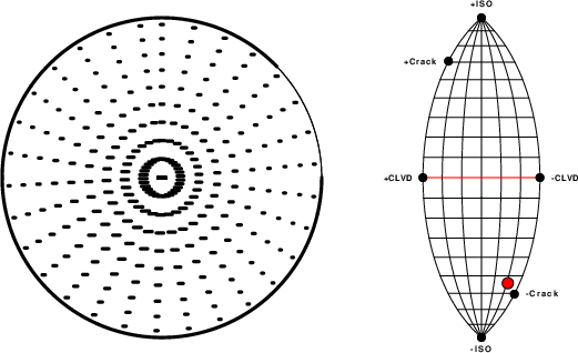
The P-wave first motion mechanism corresponding to the best fit is
|
|
|
The best fit as a function of depth is given in the following figure:

|
|
|
The comparison of the observed and predicted waveforms is given in the next figure. The red traces are the observed and the blue are the predicted. Each observed-predicted component is plotted to the same scale and peak amplitudes are indicated by the numbers to the left of each trace. A pair of numbers is given in black at the right of each predicted traces. The upper number it the time shift required for maximum correlation between the observed and predicted traces. This time shift is required because the synthetics are not computed at exactly the same distance as the observed and because the velocity model used in the predictions may not be perfect. A positive time shift indicates that the prediction is too fast and should be delayed to match the observed trace (shift to the right in this figure). A negative value indicates that the prediction is too slow. The lower number gives the percentage of variance reduction to characterize the individual goodness of fit (100% indicates a perfect fit).
The bandpass filter used in the processing and for the display was
cut o DIST/3.3 -20 o DIST/3.3 +50
rtr
taper w 0.1
hp c 0.03 n 3
lp c 0.10 n 3
|
|
|
A check on the assumed source location is possible by looking at the time shifts between the observed and predicted traces. The time shifts for waveform matching arise for several reasons:
Time_shift = A + B cos Azimuth + C Sin Azimuth
The time shifts for this inversion lead to the next figure:
The derived shift in origin time and epicentral coordinates are given at the bottom of the figure.
(Return to selection section) (Return to selection section)
The CUS.model used for the waveform synthetic seismograms and for the surface wave eigenfunctions and dispersion is as follows:
MODEL.01
CUS Model with Q from simple gamma values
ISOTROPIC
KGS
FLAT EARTH
1-D
CONSTANT VELOCITY
LINE08
LINE09
LINE10
LINE11
  H(KM) VP(KM/S) VS(KM/S) RHO(GM/CC)   QP   QS  ETAP  ETAS  FREFP  FREFS
  1.0000  5.0000  2.8900  2.5000 0.172E-02 0.387E-02 0.00  0.00  1.00  1.00
  9.0000  6.1000  3.5200  2.7300 0.160E-02 0.363E-02 0.00  0.00  1.00  1.00
 10.0000  6.4000  3.7000  2.8200 0.149E-02 0.336E-02 0.00  0.00  1.00  1.00
 20.0000  6.7000  3.8700  2.9020 0.000E-04 0.000E-04 0.00  0.00  1.00  1.00
  0.0000  8.1500  4.7000  3.3640 0.194E-02 0.431E-02 0.00  0.00  1.00  1.00
Thanks also to the many seismic network operators whose dedication make this effort possible: University of Nevada Reno, University of Alaska, University of Washington, Oregon State University, University of Utah, Montana Bureau of Mines, UC Berkeley, Caltech, Saint Louis University, University of Memphis, the Oklahoma Geological Survey, TexNet, the Iris stations and other networks.