
 USGS/SLU Moment Tensor Solution
 ENS  2021/08/13 11:57:35:0  35.88  -84.90   1.0 3.5 Tennessee

 Stations used:
   CO.CASEE CO.HODGE CO.PAULI ET.CPCT IM.TKL IU.WCI IU.WVT
   N4.R49A N4.R50A N4.S51A N4.T47A N4.T50A N4.U49A N4.V48A
   N4.V53A N4.V55A N4.W50A N4.W52A N4.X48A N4.X51A N4.Y52A
   NM.BLO NM.USIN US.GOGA US.LRAL US.TZTN

 Filtering commands used:
   cut o DIST/3.3 -40 o DIST/3.3 +50
   rtr
   taper w 0.1
   hp c 0.03 n 3
   lp c 0.10 n 3

 Best Fitting Double Couple
  Mo = 1.26e+22 dyne-cm
  Mw = 4.00
  Z  = 1 km
  Plane   Strike  Dip  Rake
   NP1       65    80    93
   NP2      230    10    75
  Principal Axes:
   Axis    Value   Plunge  Azimuth
    T   1.26e+22     55     338
    N   0.00e+00      3     245
    P  -1.26e+22     35     153

 Moment Tensor: (dyne-cm)
    Component   Value
       Mxx    -3.00e+21
       Mxy     1.95e+21
       Mxz     1.08e+22
       Myy    -1.16e+21
       Myz    -4.89e+21
       Mzz     4.16e+21


                     --------------
                 ----#################-
              ----#######################-
             --############################
           --################################
          --###########   ####################
         --############ T ####################-
        --#############   ##################----
        -#################################------
       --##############################----------
       --##########################--------------
       -########################-----------------
       -####################---------------------
        -###############------------------------
        -#########------------------------------
         -##-----------------------------------
          -----------------------   ----------
           ---------------------- P ---------
             --------------------   -------
              ----------------------------
                 ----------------------
                     --------------


 Global CMT Convention Moment Tensor:
      R          T          P
  4.16e+21   1.08e+22   4.89e+21
  1.08e+22  -3.00e+21  -1.95e+21
  4.89e+21  -1.95e+21  -1.16e+21


Details of the solution is found at

http://www.eas.slu.edu/eqc/eqc_mt/MECH.NA/20210813115735/index.html
|
      STK = 230
      DIP = 10
     RAKE = 75
       MW = 4.00
       HS = 1.0
The NDK file is 20210813115735.ndk The waveform inversion is preferred.
The following compares this source inversion to others
 USGS/SLU Moment Tensor Solution
 ENS  2021/08/13 11:57:35:0  35.88  -84.90   1.0 3.5 Tennessee

 Stations used:
   CO.CASEE CO.HODGE CO.PAULI ET.CPCT IM.TKL IU.WCI IU.WVT
   N4.R49A N4.R50A N4.S51A N4.T47A N4.T50A N4.U49A N4.V48A
   N4.V53A N4.V55A N4.W50A N4.W52A N4.X48A N4.X51A N4.Y52A
   NM.BLO NM.USIN US.GOGA US.LRAL US.TZTN

 Filtering commands used:
   cut o DIST/3.3 -40 o DIST/3.3 +50
   rtr
   taper w 0.1
   hp c 0.03 n 3
   lp c 0.10 n 3

 Best Fitting Double Couple
  Mo = 1.26e+22 dyne-cm
  Mw = 4.00
  Z  = 1 km
  Plane   Strike  Dip  Rake
   NP1       65    80    93
   NP2      230    10    75
  Principal Axes:
   Axis    Value   Plunge  Azimuth
    T   1.26e+22     55     338
    N   0.00e+00      3     245
    P  -1.26e+22     35     153

 Moment Tensor: (dyne-cm)
    Component   Value
       Mxx    -3.00e+21
       Mxy     1.95e+21
       Mxz     1.08e+22
       Myy    -1.16e+21
       Myz    -4.89e+21
       Mzz     4.16e+21


                     --------------
                 ----#################-
              ----#######################-
             --############################
           --################################
          --###########   ####################
         --############ T ####################-
        --#############   ##################----
        -#################################------
       --##############################----------
       --##########################--------------
       -########################-----------------
       -####################---------------------
        -###############------------------------
        -#########------------------------------
         -##-----------------------------------
          -----------------------   ----------
           ---------------------- P ---------
             --------------------   -------
              ----------------------------
                 ----------------------
                     --------------


 Global CMT Convention Moment Tensor:
      R          T          P
  4.16e+21   1.08e+22   4.89e+21
  1.08e+22  -3.00e+21  -1.95e+21
  4.89e+21  -1.95e+21  -1.16e+21


Details of the solution is found at

http://www.eas.slu.edu/eqc/eqc_mt/MECH.NA/20210813115735/index.html
|
 Moment (dyne-cm)   2.08E+22   dyne-cm
 Magnitude (Mw)    4.15
 Depth   1 km

 Principal Axes:
   Axis    Value   Plunge  Azimuth
    T  -4.94E+21     29.     19.
    N  -1.07E+22      1.    288.
    P  -2.69E+22     61.    197.
 Moment Tensor: (dyne-cm) Aki-Richards               Lune parameters
    Component   Value
       Mxx   -1.01E+22                                beta:  146.76
       Mxy    3.00E+20                                gamma:  15.29
       Mxz    8.80E+21
       Myy   -1.06E+22
       Myz    2.80E+21
       Mzz   -2.19E+22
 Global CMT Convention Moment Tensor: (dyne-cm)
         R         T         F
  R -2.19E+22  8.80E+21 -2.80E+21
  T  8.80E+21 -1.01E+22 -3.00E+20
  F -2.80E+21 -3.00E+20 -1.06E+22


                    --------------                         :
                ----------------------                   :---:
             -----------------   --------              ::. ..::
            ------------------ T ---------            :--------:
          --------------------   -----------         :: .  . .  :
         ------------------------------------        :  .  .  .  :
        --------------------------------------      :------------::
       ----------------------------------------    ::  .   .  .   :
       ----------------------------------------    :   .   .   .  :
      ------------------------------------------   :---------------:
      ------------------------------------------   :   .   .   .   :
      ------------------------------------------   :===============:
      ------------------------------------------   :   .   .   .   :
       ----------------   ---------------------    :   .   .   .   :
       ---------------- P ---------------------    :---------------:
        ---------------   --------------------     :   .   .   .  :
         ------------------------------------      ::  .   .  .   :
          ----------------------------------        :------------::
            ------------------------------           :  .  .  .  :
             ----------------------------            :: .  . #  :
                ----------------------                :--------:
                    --------------                     ::. ..::
                                                         :---:
                                                           :
|
 Moment (dyne-cm)   1.26E+22   dyne-cm
 Magnitude (Mw)    4.00
 Depth   1.0 km

 Principal Axes:
   Axis    Value   Plunge  Azimuth
    T   1.26E+22     55.    338.
    N   7.07E+17      3.    245.
    P  -1.26E+22     35.    153.
 Moment Tensor: (dyne-cm) Aki-Richards               Lune parameters
    Component   Value
       Mxx   -3.01E+21                                beta:   90.00
       Mxy    1.95E+21                                gamma:   0.00
       Mxz    1.08E+22
       Myy   -1.16E+21
       Myz   -4.90E+21
       Mzz    4.17E+21
 Global CMT Convention Moment Tensor: (dyne-cm)
         R         T         F
  R  4.17E+21  1.08E+22  4.90E+21
  T  1.08E+22 -3.01E+21 -1.95E+21
  F  4.90E+21 -1.95E+21 -1.16E+21


                    --------------                         :
                ----#################-                   :---:
             ----#######################-              ::. ..::
            --############################            :--------:
          --################################         :: .  . .  :
         --###########   ####################        :  .  .  .  :
        --############ T ####################-      :------------::
       --#############   ##################----    ::  .   .  .   :
       -#################################------    :   .   .   .  :
      --##############################----------   :---------------:
      --##########################--------------   :   .   .   .   :
      -########################-----------------   :=======#=======:
      -####################---------------------   :   .   .   .   :
       -###############------------------------    :   .   .   .   :
       -##########-----------------------------    :---------------:
        -##-----------------------------------     :   .   .   .  :
         -----------------------   ----------      ::  .   .  .   :
          ---------------------- P ---------        :------------::
            --------------------   -------           :  .  .  .  :
             ----------------------------            :: .  . .  :
                ----------------------                :--------:
                    --------------                     ::. ..::
                                                         :---:
                                                           :
|
 Moment (dyne-cm)   1.40E+22   dyne-cm
 Magnitude (Mw)    4.03
 Depth   1.0 km

 Principal Axes:
   Axis    Value   Plunge  Azimuth
    T   1.55E+22     55.      7.
    N  -3.86E+21      2.    275.
    P  -1.16E+22     35.    184.
 Moment Tensor: (dyne-cm) Aki-Richards               Lune parameters
    Component   Value
       Mxx   -2.71E+21                                beta:   90.00
       Mxy    4.82E+20                                gamma: -13.85
       Mxz    1.27E+22
       Myy   -3.78E+21
       Myz    1.39E+21
       Mzz    6.49E+21
 Global CMT Convention Moment Tensor: (dyne-cm)
         R         T         F
  R  6.49E+21  1.27E+22 -1.39E+21
  T  1.27E+22 -2.71E+21 -4.82E+20
  F -1.39E+21 -4.82E+20 -3.78E+21


                    -----#####----                         :
                ---#################--                   :---:
             ---#######################--              ::. ..::
            ---##########################-            :--------:
          ---#############################--         :: .  . .  :
         ---###############   #############--        :  .  .  .  :
        ----############### T ##############--      :------------::
       -----###############   ##############---    ::  .   .  .   :
       -----################################---    :   .   .   .  :
      -------##############################-----   :---------------:
      ---------###########################------   :   .   .   .   :
      -----------########################-------   :===#===========:
      ----------------###############-----------   :   .   .   .   :
       ----------------------------------------    :   .   .   .   :
       ----------------------------------------    :---------------:
        --------------------------------------     :   .   .   .  :
         ------------------------------------      ::  .   .  .   :
          ---------------   ----------------        :------------::
            ------------- P --------------           :  .  .  .  :
             ------------   -------------            :: .  . .  :
                ----------------------                :--------:
                    --------------                     ::. ..::
                                                         :---:
                                                           :
|
 Moment (dyne-cm)   1.72E+22   dyne-cm
 Magnitude (Mw)    4.09
 Depth   1.0 km

 Principal Axes:
   Axis    Value   Plunge  Azimuth
    T  -2.01E+21     35.     20.
    N  -9.33E+21     -0.    290.
    P  -2.24E+22     55.    200.
 Moment Tensor: (dyne-cm) Aki-Richards               Lune parameters
    Component   Value
       Mxx   -8.78E+21                                beta:  143.14
       Mxy    2.01E+20                                gamma:   9.23
       Mxz    9.00E+21
       Myy   -9.26E+21
       Myz    3.27E+21
       Mzz   -1.57E+22
 Global CMT Convention Moment Tensor: (dyne-cm)
         R         T         F
  R -1.57E+22  9.00E+21 -3.27E+21
  T  9.00E+21 -8.78E+21 -2.01E+20
  F -3.27E+21 -2.01E+20 -9.26E+21


                    --------------                         :
                ----------------------                   :---:
             ----------------------------              ::. ..::
            ------------------   ---------            :--------:
          -------------------- T -----------         :: .  . .  :
         ---------------------   ------------        :  .  .  .  :
        --------------------------------------      :------------::
       ----------------------------------------    ::  .   .  .   :
       ----------------------------------------    :   .   .   .  :
      ------------------------------------------   :---------------:
      ------------------------------------------   :   .   .   .   :
      ------------------------------------------   :===============:
      ------------------------------------------   :   .   .   .   :
       ----------------------------------------    :   .   .   .   :
       ---------------   ----------------------    :---------------:
        -------------- P ---------------------     :   .   .   .  :
         -------------   --------------------      ::  .   .  .   :
          ----------------------------------        :------------::
            ------------------------------           :  .  .  .  :
             ----------------------------            :: .  .#.  :
                ----------------------                :--------:
                    --------------                     ::. ..::
                                                         :---:
                                                           :
|
 Moment (dyne-cm)   2.08E+22   dyne-cm
 Magnitude (Mw)    4.15
 Depth   1.0 km

 Principal Axes:
   Axis    Value   Plunge  Azimuth
    T  -4.94E+21     29.     19.
    N  -1.07E+22      1.    288.
    P  -2.69E+22     61.    197.
 Moment Tensor: (dyne-cm) Aki-Richards               Lune parameters
    Component   Value
       Mxx   -1.01E+22                                beta:  146.76
       Mxy    3.00E+20                                gamma:  15.29
       Mxz    8.80E+21
       Myy   -1.06E+22
       Myz    2.80E+21
       Mzz   -2.19E+22
 Global CMT Convention Moment Tensor: (dyne-cm)
         R         T         F
  R -2.19E+22  8.80E+21 -2.80E+21
  T  8.80E+21 -1.01E+22 -3.00E+20
  F -2.80E+21 -3.00E+20 -1.06E+22


                    --------------                         :
                ----------------------                   :---:
             -----------------   --------              ::. ..::
            ------------------ T ---------            :--------:
          --------------------   -----------         :: .  . .  :
         ------------------------------------        :  .  .  .  :
        --------------------------------------      :------------::
       ----------------------------------------    ::  .   .  .   :
       ----------------------------------------    :   .   .   .  :
      ------------------------------------------   :---------------:
      ------------------------------------------   :   .   .   .   :
      ------------------------------------------   :===============:
      ------------------------------------------   :   .   .   .   :
       ----------------   ---------------------    :   .   .   .   :
       ---------------- P ---------------------    :---------------:
        ---------------   --------------------     :   .   .   .  :
         ------------------------------------      ::  .   .  .   :
          ----------------------------------        :------------::
            ------------------------------           :  .  .  .  :
             ----------------------------            :: .  . #  :
                ----------------------                :--------:
                    --------------                     ::. ..::
                                                         :---:
                                                           :
|
 Moment (dyne-cm)   1.43E+22   dyne-cm
 Magnitude (Mw)    4.04
 Depth   1.0 km

 Principal Axes:
   Axis    Value   Plunge  Azimuth
    T   1.58E+22     55.     15.
    N  -3.78E+21      1.    283.
    P  -1.20E+22     35.    192.
 Moment Tensor: (dyne-cm) Aki-Richards               Lune parameters
    Component   Value
       Mxx   -2.84E+21                                beta:   90.00
       Mxy    4.45E+20                                gamma: -13.26
       Mxz    1.27E+22
       Myy   -3.62E+21
       Myz    3.16E+21
       Mzz    6.46E+21
 Global CMT Convention Moment Tensor: (dyne-cm)
         R         T         F
  R  6.46E+21  1.27E+22 -3.16E+21
  T  1.27E+22 -2.84E+21 -4.45E+20
  F -3.16E+21 -4.45E+20 -3.62E+21


                    -----#####----                         :
                ---#################--                   :---:
             ----######################--              ::. ..::
            ---##########################-            :--------:
          ----############################--         :: .  . .  :
         ----###############   ############--        :  .  .  .  :
        -----############### T #############--      :------------::
       ------###############   #############---    ::  .   .  .   :
       ------################################--    :   .   .   .  :
      ---------#############################----   :---------------:
      -----------###########################----   :   .   .   .   :
      --------------#######################-----   :===#===========:
      ------------------################--------   :   .   .   .   :
       ----------------------------------------    :   .   .   .   :
       ----------------------------------------    :---------------:
        --------------------------------------     :   .   .   .  :
         ------------------------------------      ::  .   .  .   :
          -------------   ------------------        :------------::
            ----------- P ----------------           :  .  .  .  :
             ----------   ---------------            :: .  . .  :
                ----------------------                :--------:
                    --------------                     ::. ..::
                                                         :---:
                                                           :
|
|
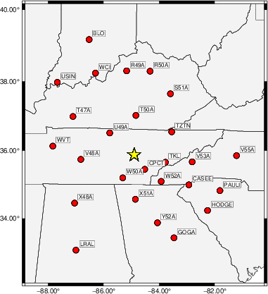
The focal mechanism was determined using broadband seismic waveforms. The location of the event and the and stations used for the waveform inversion are shown in the next figure.
|
|
|
The program wvfgrd96 was used with good traces observed at short distance to determine the focal mechanism, depth and seismic moment. This technique requires a high quality signal and well determined velocity model for the Green functions. To the extent that these are the quality data, this type of mechanism should be preferred over the radiation pattern technique which requires the separate step of defining the pressure and tension quadrants and the correct strike.
The observed and predicted traces are filtered using the following gsac commands:
cut o DIST/3.3 -40 o DIST/3.3 +50
rtr
taper w 0.1
hp c 0.03 n 3
lp c 0.10 n 3
The results of this grid search from 0.5 to 19 km depth are as follow:
           DEPTH  STK   DIP  RAKE   MW    FIT
WVFGRD96    1.0   230    10    75   4.00 0.7748
WVFGRD96    2.0   230    15    75   3.89 0.7145
WVFGRD96    3.0   230    15    75   3.83 0.6444
WVFGRD96    4.0   220    15    65   3.78 0.5976
WVFGRD96    5.0   200    15    45   3.75 0.5721
The best solution is
WVFGRD96 1.0 230 10 75 4.00 0.7748
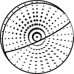
The mechanism correspond to the best fit is
|
|
|
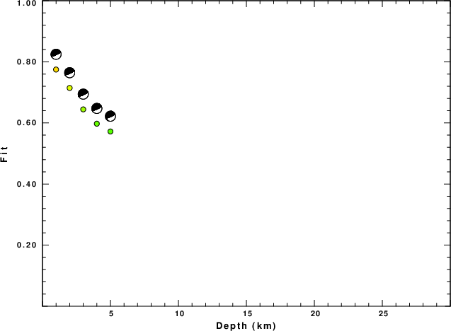
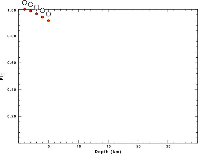
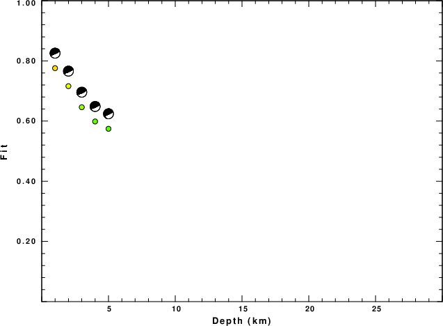
The best fit as a function of depth is given in the following figure:
|
|
|
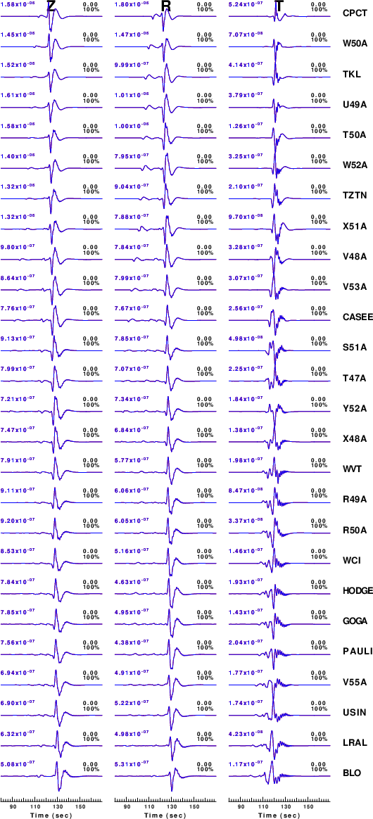
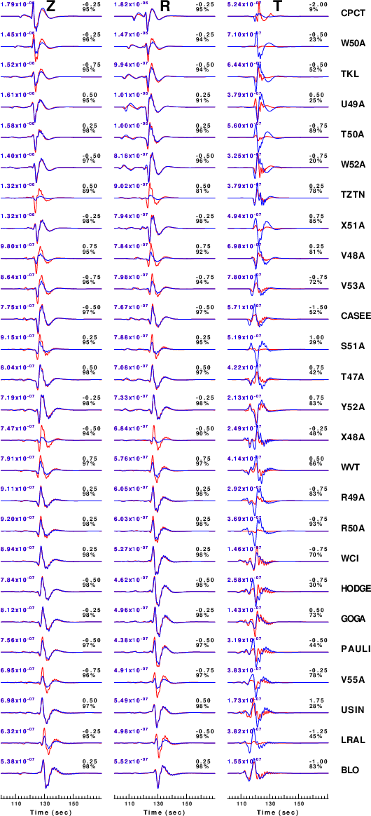
The comparison of the observed and predicted waveforms is given in the next figure. The red traces are the observed and the blue are the predicted. Each observed-predicted component is plotted to the same scale and peak amplitudes are indicated by the numbers to the left of each trace. A pair of numbers is given in black at the right of each predicted traces. The upper number it the time shift required for maximum correlation between the observed and predicted traces. This time shift is required because the synthetics are not computed at exactly the same distance as the observed and because the velocity model used in the predictions may not be perfect. A positive time shift indicates that the prediction is too fast and should be delayed to match the observed trace (shift to the right in this figure). A negative value indicates that the prediction is too slow. The lower number gives the percentage of variance reduction to characterize the individual goodness of fit (100% indicates a perfect fit).
The bandpass filter used in the processing and for the display was
cut o DIST/3.3 -40 o DIST/3.3 +50
rtr
taper w 0.1
hp c 0.03 n 3
lp c 0.10 n 3

|
|
|
|
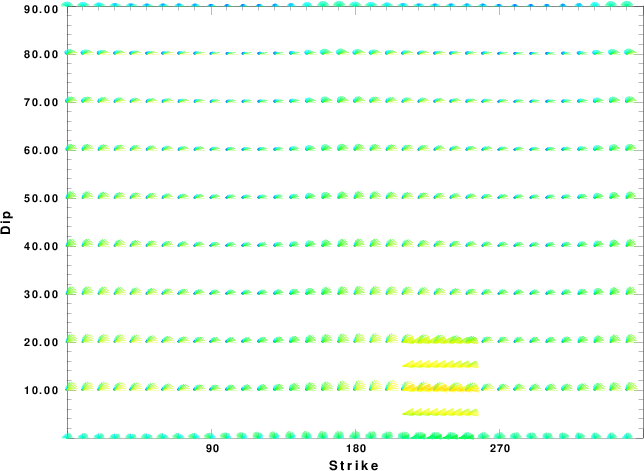
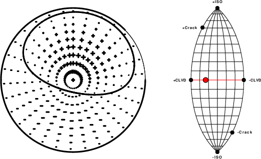
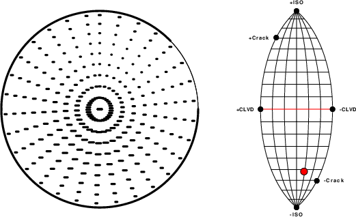
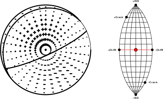
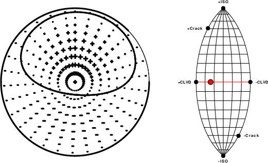
| Focal mechanism sensitivity at the preferred depth. The red color indicates a very good fit to thewavefroms. Each solution is plotted as a vector at a given value of strike and dip with the angle of the vector representing the rake angle, measured, with respect to the upward vertical (N) in the figure. |
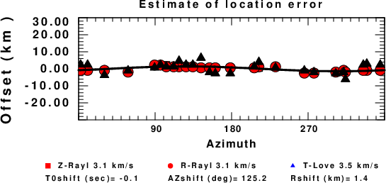
A check on the assumed source location is possible by looking at the time shifts between the observed and predicted traces. The time shifts for waveform matching arise for several reasons:
Time_shift = A + B cos Azimuth + C Sin Azimuth
The time shifts for this inversion lead to the next figure:

The derived shift in origin time and epicentral coordinates are given at the bottom of the figure.
The focal mechanism was determined using broadband seismic waveforms. The location of the event and the and stations used for the waveform inversion are shown in the next figure.

|
|
|
The program wvfmtd96 was used with good traces observed at short distance to determine the focal mechanism, depth and seismic moment. This technique requires a high quality signal and well determined velocity model for the Green functions. To the extent that these are the quality data, this type of mechanism should be preferred over the radiation pattern technique which requires the separate step of defining the pressure and tension quadrants and the correct strike.
The observed and predicted traces are filtered using the following gsac commands:
cut o DIST/3.3 -40 o DIST/3.3 +50
rtr
taper w 0.1
hp c 0.03 n 3
lp c 0.10 n 3
The results of this grid search over depth are as follow:
MT Program H(km)                    Mw                           Fit                              Mxx(dyne-cm)    Myy           Mxy            Mxz            Myz            Mzz
WVFMTD961    1.0  103.   80.   91.   4.04     0.930 0.318E-07     0.928     0.964 0.253E-07  47.9 -0.2843026E+22 -0.3620183E+22  0.4454430E+21  0.1273254E+23  0.3155309E+22  0.6463209E+22
WVFMTD961    2.0  104.   73.   93.   3.95     0.790 0.550E-07     0.779     0.889 0.444E-07  74.5 -0.3482789E+22 -0.4207324E+22  0.6089934E+21  0.7724496E+22  0.2375683E+22  0.7690113E+22
WVFMTD961    3.0  100.   73.   98.   3.89     0.633 0.729E-07     0.619     0.796 0.584E-07  77.8 -0.2694129E+22 -0.3316760E+22  0.1034962E+22  0.6207957E+22  0.2232103E+22  0.6010889E+22
WVFMTD961    4.0  296.   62.  -98.   3.81     0.346 0.971E-07     0.349     0.588 0.762E-07  46.5  0.3346578E+22  0.2677260E+22  0.1508864E+22  0.3421390E+22  0.8482498E+21 -0.6023838E+22
WVFMTD961    5.0  302.   53.  -93.   3.88     0.527 0.825E-07     0.521     0.726 0.653E-07  73.9  0.4819937E+22  0.4195446E+22  0.1045229E+22  0.2058308E+22  0.6715092E+21 -0.9015383E+22
The best solution is
WVFMTD961 1.0 103. 80. 91. 4.04 0.930 0.318E-07 0.928 0.964 0.253E-07 47.9 -0.2843026E+22 -0.3620183E+22 0.4454430E+21 0.1273254E+23 0.3155309E+22 0.6463209E+22
The complete moment tensor decomposition using the program mtdinfo is given in the text file MTDinfo.txt. (Jost, M. L., and R. B. Herrmann (1989). A student's guide to and review of moment tensors, Seism. Res. Letters 60, 37-57. SRL_60_2_37-57.pdf.
The P-wave first motion mechanism corresponding to the best fit is
|
|
|
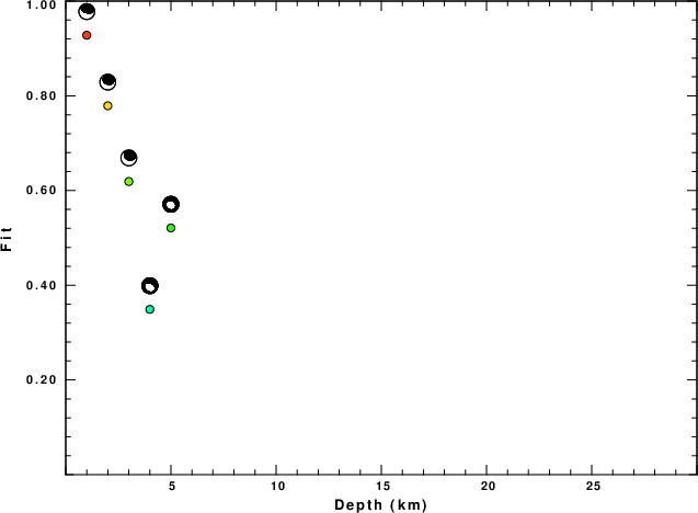
The best fit as a function of depth is given in the following figure:
|
|
|
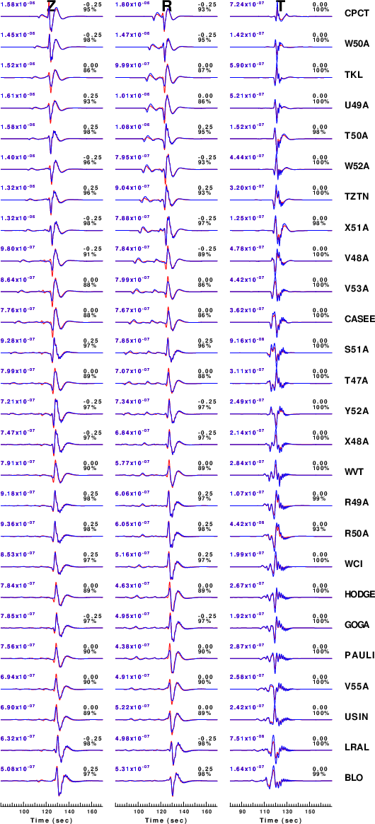
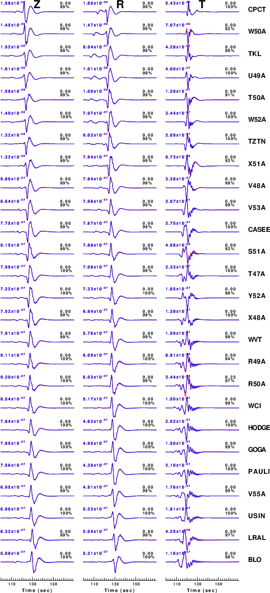
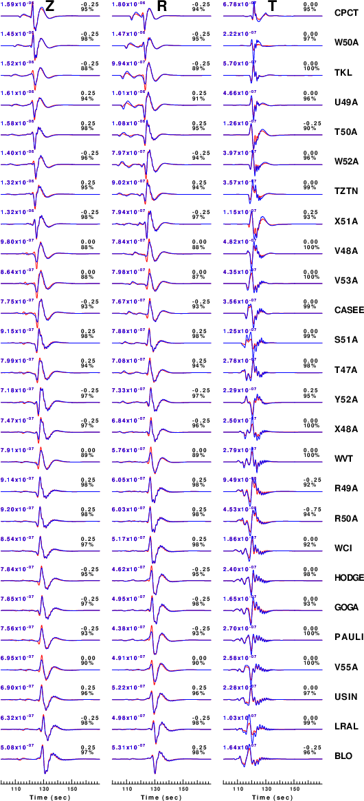
The comparison of the observed and predicted waveforms is given in the next figure. The red traces are the observed and the blue are the predicted. Each observed-predicted component is plotted to the same scale and peak amplitudes are indicated by the numbers to the left of each trace. A pair of numbers is given in black at the right of each predicted traces. The upper number it the time shift required for maximum correlation between the observed and predicted traces. This time shift is required because the synthetics are not computed at exactly the same distance as the observed and because the velocity model used in the predictions may not be perfect. A positive time shift indicates that the prediction is too fast and should be delayed to match the observed trace (shift to the right in this figure). A negative value indicates that the prediction is too slow. The lower number gives the percentage of variance reduction to characterize the individual goodness of fit (100% indicates a perfect fit).
The bandpass filter used in the processing and for the display was
cut o DIST/3.3 -40 o DIST/3.3 +50
rtr
taper w 0.1
hp c 0.03 n 3
lp c 0.10 n 3
|
|
|
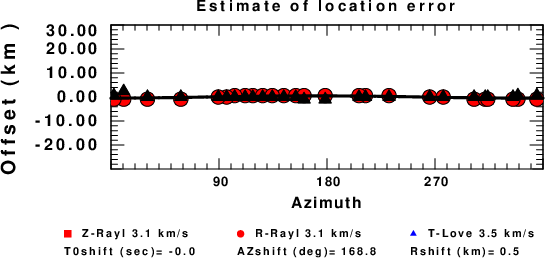
A check on the assumed source location is possible by looking at the time shifts between the observed and predicted traces. The time shifts for waveform matching arise for several reasons:
Time_shift = A + B cos Azimuth + C Sin Azimuth
The time shifts for this inversion lead to the next figure:

The derived shift in origin time and epicentral coordinates are given at the bottom of the figure.
The focal mechanism was determined using broadband seismic waveforms. The location of the event and the and stations used for the waveform inversion are shown in the next figure.

|
|
|
The program wvfmt96 was used with good traces observed at short distance to determine the focal mechanism, depth and seismic moment. This technique requires a high quality signal and well determined velocity model for the Green functions. To the extent that these are the quality data, this type of mechanism should be preferred over the radiation pattern technique which requires the separate step of defining the pressure and tension quadrants and the correct strike.
The observed and predicted traces are filtered using the following gsac commands:
cut o DIST/3.3 -40 o DIST/3.3 +50
rtr
taper w 0.1
hp c 0.03 n 3
lp c 0.10 n 3
The results of this grid search over depth are as follow:
MT Program H(km)                    Mw                           Fit                              Mxx(dyne-cm)    Myy           Mxy            Mxz            Myz            Mzz
WVFMT961    1.0  288.   74.  -91.   4.15     1.000 0.184E-12     1.000     1.000 0.147E-12  54.5 -0.1010000E+23 -0.1060000E+23  0.3000005E+21  0.8799995E+22  0.2799998E+22 -0.2190000E+23
WVFMT961    2.0  290.   65.  -91.   4.08     0.988 0.133E-07     0.987     0.994 0.107E-07  68.8 -0.8465412E+22 -0.9118889E+22  0.3790051E+21  0.4120273E+22  0.1348096E+22 -0.1872178E+23
WVFMT961    3.0  290.   61.  -91.   4.05     0.968 0.214E-07     0.967     0.984 0.172E-07  71.5 -0.7464658E+22 -0.8292816E+22  0.4225719E+21  0.2987755E+22  0.9642471E+21 -0.1741766E+23
WVFMT961    4.0  291.   59.  -91.   4.03     0.944 0.283E-07     0.942     0.972 0.227E-07  73.1 -0.6713553E+22 -0.7515828E+22  0.4639834E+21  0.2481360E+22  0.7933492E+21 -0.1647908E+23
WVFMT961    5.0  291.   58.  -91.   4.01     0.918 0.343E-07     0.915     0.958 0.275E-07  75.8 -0.6053040E+22 -0.6824195E+22  0.4018019E+21  0.2201268E+22  0.6953245E+21 -0.1570855E+23
The best solution is
WVFMT961 1.0 288. 74. -91. 4.15 1.000 0.184E-12 1.000 1.000 0.147E-12 54.5 -0.1010000E+23 -0.1060000E+23 0.3000005E+21 0.8799995E+22 0.2799998E+22 -0.2190000E+23
The complete moment tensor decomposition using the program mtinfo is given in the text file MTinfo.txt. (Jost, M. L., and R. B. Herrmann (1989). A student's guide to and review of moment tensors, Seism. Res. Letters 60, 37-57. SRL_60_2_37-57.pdf.
The P-wave first motion mechanism corresponding to the best fit is
|
|
|
The best fit as a function of depth is given in the following figure:
|
|
|
The comparison of the observed and predicted waveforms is given in the next figure. The red traces are the observed and the blue are the predicted. Each observed-predicted component is plotted to the same scale and peak amplitudes are indicated by the numbers to the left of each trace. A pair of numbers is given in black at the right of each predicted traces. The upper number it the time shift required for maximum correlation between the observed and predicted traces. This time shift is required because the synthetics are not computed at exactly the same distance as the observed and because the velocity model used in the predictions may not be perfect. A positive time shift indicates that the prediction is too fast and should be delayed to match the observed trace (shift to the right in this figure). A negative value indicates that the prediction is too slow. The lower number gives the percentage of variance reduction to characterize the individual goodness of fit (100% indicates a perfect fit).
The bandpass filter used in the processing and for the display was
cut o DIST/3.3 -40 o DIST/3.3 +50
rtr
taper w 0.1
hp c 0.03 n 3
lp c 0.10 n 3
|
|
|
A check on the assumed source location is possible by looking at the time shifts between the observed and predicted traces. The time shifts for waveform matching arise for several reasons:
Time_shift = A + B cos Azimuth + C Sin Azimuth
The time shifts for this inversion lead to the next figure:

The derived shift in origin time and epicentral coordinates are given at the bottom of the figure.
The focal mechanism was determined using broadband seismic waveforms. The location of the event and the and stations used for the waveform inversion are shown in the next figure.

|
|
|
The program wvfmtgrd96 was used with good traces observed at short distance to determine the focal mechanism, depth and seismic moment. This technique requires a high quality signal and well determined velocity model for the Green functions. To the extent that these are the quality data, this type of mechanism should be preferred over the radiation pattern technique which requires the separate step of defining the pressure and tension quadrants and the correct strike.
The observed and predicted traces are filtered using the following gsac commands:
cut o DIST/3.3 -20 o DIST/3.3 +50
rtr
taper w 0.1
hp c 0.03 n 3
lp c 0.10 n 3
The results of this grid search over depth are as follow:
MT Program  H(km) Mxx(dyne-cm)   Myy        Mxy        Mxz        Myz        Mzz       Mw      Fit
WVFMTGRD96    1.0 -0.878E+22 -0.926E+22  0.201E+21  0.900E+22  0.327E+22 -0.157E+23  4.0904  0.9935
WVFMTGRD96    2.0 -0.832E+22 -0.909E+22  0.324E+21  0.435E+22  0.158E+22 -0.192E+23  4.0837  0.9861
WVFMTGRD96    3.0 -0.721E+22 -0.779E+22  0.587E+21  0.310E+22  0.101E+22 -0.180E+23  4.0529  0.9663
WVFMTGRD96    4.0 -0.689E+22 -0.736E+22  0.197E+21  0.261E+22  0.952E+21 -0.165E+23  4.0293  0.9418
WVFMTGRD96    5.0 -0.567E+22 -0.682E+22  0.685E+21  0.890E+21  0.415E+21 -0.165E+23  4.0158  0.9163
The best solution is
WVFMTGRD96 1.0 -0.878E+22 -0.926E+22 0.201E+21 0.900E+22 0.327E+22 -0.157E+23 4.0904 0.9935
The complete moment tensor decomposition using the program mtinfo is given in the text file MTGRDinfo.txt. (Jost, M. L., and R. B. Herrmann (1989). A student's guide to and review of moment tensors, Seism. Res. Letters 60, 37-57. SRL_60_2_37-57.pdf.
The P-wave first motion mechanism corresponding to the best fit is
|
|
|
The best fit as a function of depth is given in the following figure:

|
|
|
The comparison of the observed and predicted waveforms is given in the next figure. The red traces are the observed and the blue are the predicted. Each observed-predicted component is plotted to the same scale and peak amplitudes are indicated by the numbers to the left of each trace. A pair of numbers is given in black at the right of each predicted traces. The upper number it the time shift required for maximum correlation between the observed and predicted traces. This time shift is required because the synthetics are not computed at exactly the same distance as the observed and because the velocity model used in the predictions may not be perfect. A positive time shift indicates that the prediction is too fast and should be delayed to match the observed trace (shift to the right in this figure). A negative value indicates that the prediction is too slow. The lower number gives the percentage of variance reduction to characterize the individual goodness of fit (100% indicates a perfect fit).
The bandpass filter used in the processing and for the display was
cut o DIST/3.3 -20 o DIST/3.3 +50
rtr
taper w 0.1
hp c 0.03 n 3
lp c 0.10 n 3
|
|
|
A check on the assumed source location is possible by looking at the time shifts between the observed and predicted traces. The time shifts for waveform matching arise for several reasons:
Time_shift = A + B cos Azimuth + C Sin Azimuth
The time shifts for this inversion lead to the next figure:

The derived shift in origin time and epicentral coordinates are given at the bottom of the figure.
The focal mechanism was determined using broadband seismic waveforms. The location of the event and the and stations used for the waveform inversion are shown in the next figure.

|
|
|
The program wvfmtgrd96 was used with good traces observed at short distance to determine the focal mechanism, depth and seismic moment. This technique requires a high quality signal and well determined velocity model for the Green functions. To the extent that these are the quality data, this type of mechanism should be preferred over the radiation pattern technique which requires the separate step of defining the pressure and tension quadrants and the correct strike.
The observed and predicted traces are filtered using the following gsac commands:
cut o DIST/3.3 -20 o DIST/3.3 +50
rtr
taper w 0.1
hp c 0.03 n 3
lp c 0.10 n 3
The results of this grid search over depth are as follow:
MT Program  H(km) Mxx(dyne-cm)   Myy        Mxy        Mxz        Myz        Mzz       Mw      Fit
WVFMTGRD96    1.0 -0.301E+22 -0.116E+22  0.195E+22  0.108E+23 -0.490E+22  0.417E+22  4.0007  0.7758
WVFMTGRD96    2.0 -0.298E+22 -0.114E+22  0.193E+22  0.685E+22 -0.296E+22  0.412E+22  3.8876  0.7161
WVFMTGRD96    3.0 -0.243E+22 -0.927E+21  0.157E+22  0.556E+22 -0.240E+22  0.335E+22  3.8277  0.6461
WVFMTGRD96    4.0 -0.208E+22 -0.927E+21  0.148E+22  0.478E+22 -0.208E+22  0.301E+22  3.7873  0.5987
WVFMTGRD96    5.0 -0.778E+21 -0.102E+22  0.128E+22  0.455E+22 -0.194E+22  0.180E+22  3.7516  0.5744
The best solution is
WVFMTGRD96 1.0 -0.301E+22 -0.116E+22 0.195E+22 0.108E+23 -0.490E+22 0.417E+22 4.0007 0.7758
The complete moment tensor decomposition using the program mtinfo is given in the text file MTGRDDCinfo.txt. (Jost, M. L., and R. B. Herrmann (1989). A student's guide to and review of moment tensors, Seism. Res. Letters 60, 37-57. SRL_60_2_37-57.pdf.
The P-wave first motion mechanism corresponding to the best fit is
|
|
|
The best fit as a function of depth is given in the following figure:
|
|
|
The comparison of the observed and predicted waveforms is given in the next figure. The red traces are the observed and the blue are the predicted. Each observed-predicted component is plotted to the same scale and peak amplitudes are indicated by the numbers to the left of each trace. A pair of numbers is given in black at the right of each predicted traces. The upper number it the time shift required for maximum correlation between the observed and predicted traces. This time shift is required because the synthetics are not computed at exactly the same distance as the observed and because the velocity model used in the predictions may not be perfect. A positive time shift indicates that the prediction is too fast and should be delayed to match the observed trace (shift to the right in this figure). A negative value indicates that the prediction is too slow. The lower number gives the percentage of variance reduction to characterize the individual goodness of fit (100% indicates a perfect fit).
The bandpass filter used in the processing and for the display was
cut o DIST/3.3 -20 o DIST/3.3 +50
rtr
taper w 0.1
hp c 0.03 n 3
lp c 0.10 n 3
|
|
|
A check on the assumed source location is possible by looking at the time shifts between the observed and predicted traces. The time shifts for waveform matching arise for several reasons:
Time_shift = A + B cos Azimuth + C Sin Azimuth
The time shifts for this inversion lead to the next figure:
The derived shift in origin time and epicentral coordinates are given at the bottom of the figure.
The focal mechanism was determined using broadband seismic waveforms. The location of the event and the and stations used for the waveform inversion are shown in the next figure.

|
|
|
The program wvfmtgrd96 was used with good traces observed at short distance to determine the focal mechanism, depth and seismic moment. This technique requires a high quality signal and well determined velocity model for the Green functions. To the extent that these are the quality data, this type of mechanism should be preferred over the radiation pattern technique which requires the separate step of defining the pressure and tension quadrants and the correct strike.
The observed and predicted traces are filtered using the following gsac commands:
cut o DIST/3.3 -20 o DIST/3.3 +50
rtr
taper w 0.1
hp c 0.03 n 3
lp c 0.10 n 3
The results of this grid search over depth are as follow:
MT Program  H(km) Mxx(dyne-cm)   Myy        Mxy        Mxz        Myz        Mzz       Mw      Fit
WVFMTGRD96    1.0 -0.271E+22 -0.378E+22  0.482E+21  0.127E+23  0.139E+22  0.649E+22  4.0298  0.9366
WVFMTGRD96    2.0 -0.385E+22 -0.434E+22  0.380E+21  0.730E+22 -0.196E+22  0.819E+22  3.9439  0.8458
WVFMTGRD96    3.0 -0.323E+22 -0.365E+22  0.319E+21  0.613E+22 -0.165E+22  0.688E+22  3.8935  0.7199
WVFMTGRD96    4.0 -0.252E+22 -0.288E+22  0.529E+21  0.503E+22 -0.166E+22  0.540E+22  3.8337  0.6308
WVFMTGRD96    5.0 -0.118E+22 -0.185E+22  0.620E+21  0.471E+22 -0.165E+22  0.303E+22  3.7697  0.5853
The best solution is
WVFMTGRD96 1.0 -0.271E+22 -0.378E+22 0.482E+21 0.127E+23 0.139E+22 0.649E+22 4.0298 0.9366
The complete moment tensor decomposition using the program mtinfo is given in the text file MTGRDDEVinfo.txt. (Jost, M. L., and R. B. Herrmann (1989). A student's guide to and review of moment tensors, Seism. Res. Letters 60, 37-57. SRL_60_2_37-57.pdf.
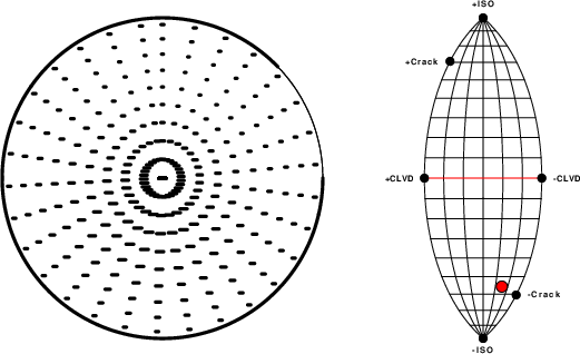
The P-wave first motion mechanism corresponding to the best fit is
|
|
|
The best fit as a function of depth is given in the following figure:

|
|
|
The comparison of the observed and predicted waveforms is given in the next figure. The red traces are the observed and the blue are the predicted. Each observed-predicted component is plotted to the same scale and peak amplitudes are indicated by the numbers to the left of each trace. A pair of numbers is given in black at the right of each predicted traces. The upper number it the time shift required for maximum correlation between the observed and predicted traces. This time shift is required because the synthetics are not computed at exactly the same distance as the observed and because the velocity model used in the predictions may not be perfect. A positive time shift indicates that the prediction is too fast and should be delayed to match the observed trace (shift to the right in this figure). A negative value indicates that the prediction is too slow. The lower number gives the percentage of variance reduction to characterize the individual goodness of fit (100% indicates a perfect fit).
The bandpass filter used in the processing and for the display was
cut o DIST/3.3 -20 o DIST/3.3 +50
rtr
taper w 0.1
hp c 0.03 n 3
lp c 0.10 n 3
|
|
|
A check on the assumed source location is possible by looking at the time shifts between the observed and predicted traces. The time shifts for waveform matching arise for several reasons:
Time_shift = A + B cos Azimuth + C Sin Azimuth
The time shifts for this inversion lead to the next figure:
The derived shift in origin time and epicentral coordinates are given at the bottom of the figure.
(Return to selection section) (Return to selection section)
The CUS.model used for the waveform synthetic seismograms and for the surface wave eigenfunctions and dispersion is as follows:
MODEL.01
CUS Model with Q from simple gamma values
ISOTROPIC
KGS
FLAT EARTH
1-D
CONSTANT VELOCITY
LINE08
LINE09
LINE10
LINE11
  H(KM) VP(KM/S) VS(KM/S) RHO(GM/CC)   QP   QS  ETAP  ETAS  FREFP  FREFS
  1.0000  5.0000  2.8900  2.5000 0.172E-02 0.387E-02 0.00  0.00  1.00  1.00
  9.0000  6.1000  3.5200  2.7300 0.160E-02 0.363E-02 0.00  0.00  1.00  1.00
 10.0000  6.4000  3.7000  2.8200 0.149E-02 0.336E-02 0.00  0.00  1.00  1.00
 20.0000  6.7000  3.8700  2.9020 0.000E-04 0.000E-04 0.00  0.00  1.00  1.00
  0.0000  8.1500  4.7000  3.3640 0.194E-02 0.431E-02 0.00  0.00  1.00  1.00
Thanks also to the many seismic network operators whose dedication make this effort possible: University of Nevada Reno, University of Alaska, University of Washington, Oregon State University, University of Utah, Montana Bureau of Mines, UC Berkeley, Caltech, Saint Louis University, University of Memphis, the Oklahoma Geological Survey, TexNet, the Iris stations and other networks.