Location
SLU Location
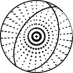
Because of the rarity of an event at this location, first motions and arrival times were read
in the 1 - 3 Hz band from the ground velocities. The program elocate was run with the CUS velocity model to determine takeoff angles to compare the first motions to the RMT solution. The output of this run is located int he file elocate.txt. The comparison between the RMT nodal planes and the first motions are shown below. There is good agreement. Many of the poor observations were along the nodal planes.
Location ANSS
2020/11/08 14:10:07 41.526 -70.966 15.1 4.0 Massachusetts
Focal Mechanism
 USGS/SLU Moment Tensor Solution
 ENS  2020/11/08 14:10:07:0  41.53  -70.97  15.1 4.0 Massachusetts

 Stations used:
   IU.HRV LD.BRNJ LD.FLET LD.KSCT LD.MCVT LD.NCB LD.ODNJ
   LD.PAL LD.UNH N4.H62A N4.J59A N4.J61A N4.K62A N4.L61B
   N4.L64A N4.M63A N4.N62A NE.BCX NE.TRY NE.WES NE.WSPT
   US.LBNH

 Filtering commands used:
   cut o DIST/3.3 -40 o DIST/3.3 +50
   rtr
   taper w 0.1
   hp c 0.03 n 3
   lp c 0.10 n 3
   br c 0.12 0.25 n 4 p 2

 Best Fitting Double Couple
  Mo = 3.39e+21 dyne-cm
  Mw = 3.62
  Z  = 7 km
  Plane   Strike  Dip  Rake
   NP1      214    52   102
   NP2       15    40    75
  Principal Axes:
   Axis    Value   Plunge  Azimuth
    T   3.39e+21     79     174
    N   0.00e+00     10      27
    P  -3.39e+21      6     296

 Moment Tensor: (dyne-cm)
    Component   Value
       Mxx    -4.98e+20
       Mxy     1.29e+21
       Mxz    -7.96e+20
       Myy    -2.73e+21
       Myz     3.75e+20
       Mzz     3.22e+21


                     -------------#
                 -------------------###
              ------------------#####-----
             ----------------#########-----
           ---------------#############------
            ------------################------
          P ----------##################-------
        -   ---------####################-------
        -----------######################-------
       -----------#######################--------
       ----------########################--------
       ----------##########   ##########---------
       ---------########### T ##########---------
        --------###########   ##########--------
        -------########################---------
         ------#######################---------
          -----######################---------
           ----#####################---------
             --###################---------
              --################----------
                 #############---------
                     ####----------


 Global CMT Convention Moment Tensor:
      R          T          P
  3.22e+21  -7.96e+20  -3.75e+20
 -7.96e+20  -4.98e+20  -1.29e+21
 -3.75e+20  -1.29e+21  -2.73e+21


Details of the solution is found at

http://www.eas.slu.edu/eqc/eqc_mt/MECH.NA/20201108141007/index.html
|
Preferred Solution
The preferred solution from an analysis of the surface-wave spectral amplitude radiation pattern, waveform inversion and first motion observations is
      STK = 15
      DIP = 40
     RAKE = 75
       MW = 3.62
       HS = 7.0
The NDK file is 20201108141007.ndk
The waveform inversion is preferred.
Moment Tensor Comparison
The following compares this source inversion to others
| SLU |
USGSMWR |
SLUFM |
 USGS/SLU Moment Tensor Solution
 ENS  2020/11/08 14:10:07:0  41.53  -70.97  15.1 4.0 Massachusetts

 Stations used:
   IU.HRV LD.BRNJ LD.FLET LD.KSCT LD.MCVT LD.NCB LD.ODNJ
   LD.PAL LD.UNH N4.H62A N4.J59A N4.J61A N4.K62A N4.L61B
   N4.L64A N4.M63A N4.N62A NE.BCX NE.TRY NE.WES NE.WSPT
   US.LBNH

 Filtering commands used:
   cut o DIST/3.3 -40 o DIST/3.3 +50
   rtr
   taper w 0.1
   hp c 0.03 n 3
   lp c 0.10 n 3
   br c 0.12 0.25 n 4 p 2

 Best Fitting Double Couple
  Mo = 3.39e+21 dyne-cm
  Mw = 3.62
  Z  = 7 km
  Plane   Strike  Dip  Rake
   NP1      214    52   102
   NP2       15    40    75
  Principal Axes:
   Axis    Value   Plunge  Azimuth
    T   3.39e+21     79     174
    N   0.00e+00     10      27
    P  -3.39e+21      6     296

 Moment Tensor: (dyne-cm)
    Component   Value
       Mxx    -4.98e+20
       Mxy     1.29e+21
       Mxz    -7.96e+20
       Myy    -2.73e+21
       Myz     3.75e+20
       Mzz     3.22e+21


                     -------------#
                 -------------------###
              ------------------#####-----
             ----------------#########-----
           ---------------#############------
            ------------################------
          P ----------##################-------
        -   ---------####################-------
        -----------######################-------
       -----------#######################--------
       ----------########################--------
       ----------##########   ##########---------
       ---------########### T ##########---------
        --------###########   ##########--------
        -------########################---------
         ------#######################---------
          -----######################---------
           ----#####################---------
             --###################---------
              --################----------
                 #############---------
                     ####----------


 Global CMT Convention Moment Tensor:
      R          T          P
  3.22e+21  -7.96e+20  -3.75e+20
 -7.96e+20  -4.98e+20  -1.29e+21
 -3.75e+20  -1.29e+21  -2.73e+21


Details of the solution is found at

http://www.eas.slu.edu/eqc/eqc_mt/MECH.NA/20201108141007/index.html
|
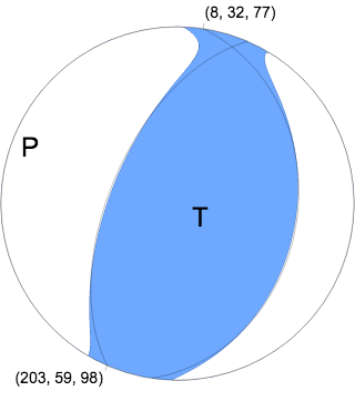
Regional Moment Tensor (Mwr)
Moment 2.987e+14 N-m
Magnitude 3.58 Mwr
Depth 7.0 km
Percent DC 91%
Half Duration -
Catalog US
Data Source US 2
Contributor US 2

Nodal Planes
Plane Strike Dip Rake
NP1 203 59 98
NP2 8 32 77

Principal Axes
Axis Value Plunge Azimuth
T 2.916e+14 N-m 75 136
N 0.137e+14 N-m 7 19
P -3.053e+14 N-m 13 288
|
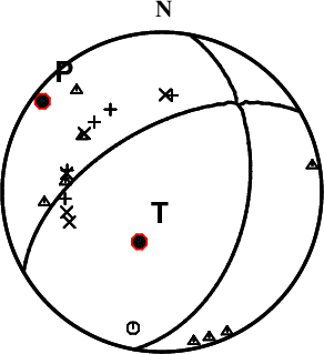
First motions and takeoff angles from an elocate run.
|
Magnitudes
mLg Magnitude
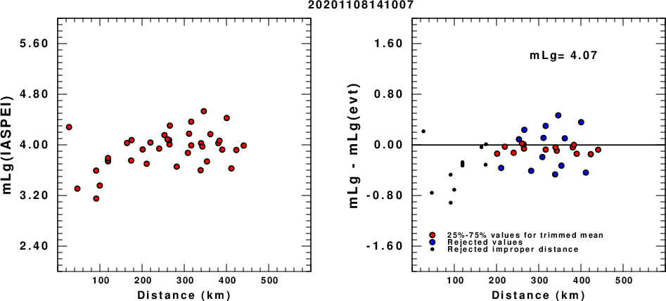
(a) mLg computed using the IASPEI formula; (b) mLg residuals ; the values used for the trimmed mean are indicated.
ML Magnitude
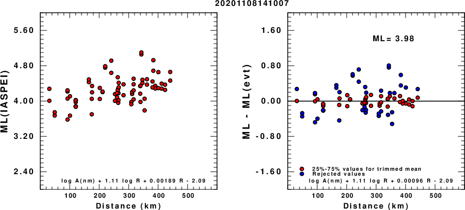
(a) ML computed using the IASPEI formula for Horizontal components; (b) ML residuals computed using a modified IASPEI formula that accounts for path specific attenuation; the values used for the trimmed mean are indicated. The ML relation used for each figure is given at the bottom of each plot.
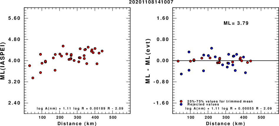
(a) ML computed using the IASPEI formula for Vertical components (research); (b) ML residuals computed using a modified IASPEI formula that accounts for path specific attenuation; the values used for the trimmed mean are indicated. The ML relation used for each figure is given at the bottom of each plot.
Context
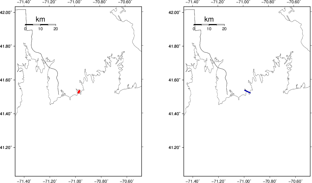
The next figure presents the focal mechanism for this earthquake (red) in the context of other events (blue) in the SLU Moment Tensor Catalog which are within ± 0.5 degrees of the new event. This comparison is shown in the left panel of the figure. The right panel shows the inferred direction of maximum compressive stress and the type of faulting (green is strike-slip, red is normal, blue is thrust; oblique is shown by a combination of colors).
Waveform Inversion using wvfgrd96
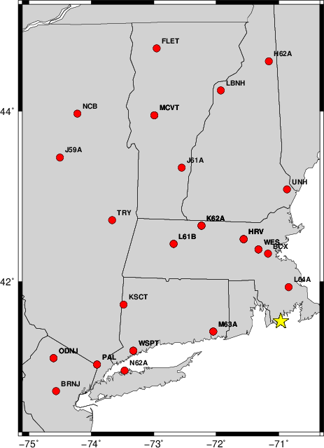
The focal mechanism was determined using broadband seismic waveforms. The location of the event and the
and stations used for the waveform inversion are shown in the next figure.
|
|
Location of broadband stations used for waveform inversion
|
The program wvfgrd96 was used with good traces observed at short distance to determine the focal mechanism, depth and seismic moment. This technique requires a high quality signal and well determined velocity model for the Green functions. To the extent that these are the quality data, this type of mechanism should be preferred over the radiation pattern technique which requires the separate step of defining the pressure and tension quadrants and the correct strike.
The observed and predicted traces are filtered using the following gsac commands:
cut o DIST/3.3 -40 o DIST/3.3 +50
rtr
taper w 0.1
hp c 0.03 n 3
lp c 0.10 n 3
br c 0.12 0.25 n 4 p 2
The results of this grid search from 0.5 to 19 km depth are as follow:
           DEPTH  STK   DIP  RAKE   MW    FIT
WVFGRD96    1.0   185    60    60   3.48 0.4580
WVFGRD96    2.0   195    60    70   3.54 0.4560
WVFGRD96    3.0   200    70    45   3.57 0.4459
WVFGRD96    4.0   340    40    20   3.52 0.4591
WVFGRD96    5.0     5    35    65   3.60 0.5039
WVFGRD96    6.0    15    35    75   3.61 0.5454
WVFGRD96    7.0    15    40    75   3.62 0.5632
WVFGRD96    8.0    15    40    75   3.61 0.5629
WVFGRD96    9.0     5    45    60   3.59 0.5533
WVFGRD96   10.0     5    45    60   3.60 0.5496
WVFGRD96   11.0     0    45    55   3.59 0.5398
WVFGRD96   12.0    -5    50    45   3.57 0.5323
WVFGRD96   13.0     0    50    50   3.58 0.5263
WVFGRD96   14.0    -5    55    45   3.58 0.5201
WVFGRD96   15.0   145    50   -45   3.59 0.5160
WVFGRD96   16.0   145    50   -40   3.59 0.5130
WVFGRD96   17.0   145    50   -40   3.59 0.5098
WVFGRD96   18.0   145    50   -40   3.60 0.5061
WVFGRD96   19.0   145    50   -40   3.61 0.5021
WVFGRD96   20.0   145    50   -40   3.63 0.5012
WVFGRD96   21.0   145    50   -40   3.63 0.4962
WVFGRD96   22.0   140    50   -45   3.65 0.4905
WVFGRD96   23.0   140    50   -45   3.65 0.4841
WVFGRD96   24.0   165    55    30   3.63 0.4786
WVFGRD96   25.0   160    55    25   3.64 0.4742
WVFGRD96   26.0   160    50    20   3.65 0.4695
WVFGRD96   27.0   160    50    20   3.66 0.4642
WVFGRD96   28.0   160    50    20   3.66 0.4588
WVFGRD96   29.0   160    50    20   3.67 0.4525
The best solution is
WVFGRD96 7.0 15 40 75 3.62 0.5632
The mechanism correspond to the best fit is
|
|
Figure 1. Waveform inversion focal mechanism
|
The best fit as a function of depth is given in the following figure:
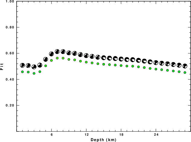
|
|
Figure 2. Depth sensitivity for waveform mechanism
|
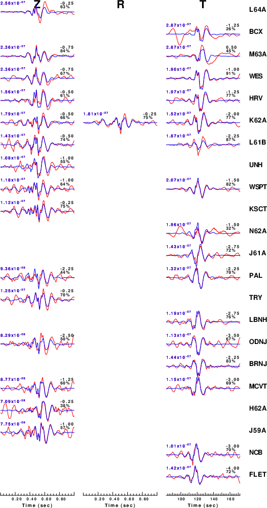
The comparison of the observed and predicted waveforms is given in the next figure. The red traces are the observed and the blue are the predicted.
Each observed-predicted component is plotted to the same scale and peak amplitudes are indicated by the numbers to the left of each trace. A pair of numbers is given in black at the right of each predicted traces. The upper number it the time shift required for maximum correlation between the observed and predicted traces. This time shift is required because the synthetics are not computed at exactly the same distance as the observed and because the velocity model used in the predictions may not be perfect.
A positive time shift indicates that the prediction is too fast and should be delayed to match the observed trace (shift to the right in this figure). A negative value indicates that the prediction is too slow. The lower number gives the percentage of variance reduction to characterize the individual goodness of fit (100% indicates a perfect fit).
The bandpass filter used in the processing and for the display was
cut o DIST/3.3 -40 o DIST/3.3 +50
rtr
taper w 0.1
hp c 0.03 n 3
lp c 0.10 n 3
br c 0.12 0.25 n 4 p 2
|
|
Figure 3. Waveform comparison for selected depth. Red: observed; Blue - predicted. The time shift with respect to the model prediction is indicated. The percent of fit is also indicated.
|
|
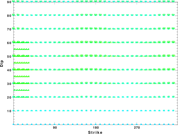
|
Focal mechanism sensitivity at the preferred depth. The red color indicates a very good fit to thewavefroms.
Each solution is plotted as a vector at a given value of strike and dip with the angle of the vector representing the rake angle, measured, with respect to the upward vertical (N) in the figure.
|
A check on the assumed source location is possible by looking at the time shifts between the observed and predicted traces. The time shifts for waveform matching arise for several reasons:
- The origin time and epicentral distance are incorrect
- The velocity model used for the inversion is incorrect
- The velocity model used to define the P-arrival time is not the
same as the velocity model used for the waveform inversion
(assuming that the initial trace alignment is based on the
P arrival time)
Assuming only a mislocation, the time shifts are fit to a functional form:
Time_shift = A + B cos Azimuth + C Sin Azimuth
The time shifts for this inversion lead to the next figure:
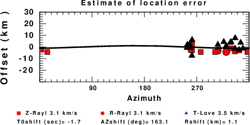
The derived shift in origin time and epicentral coordinates are given at the bottom of the figure.
Discussion
Acknowledgements
Thanks also to the many seismic network operators whose dedication make this effort possible: University of Nevada Reno, University of Alaska, University of Washington, Oregon State University, University of Utah, Montana Bureau of Mines, UC Berkely, Caltech, UC San Diego, Saint Louis University, University of Memphis, Lamont Doherty Earth Observatory, the Oklahoma Geological Survey, TexNet, the Iris stations, the Transportable Array of EarthScope and other networks.
Velocity Model
The CUS.model used for the waveform synthetic seismograms and for the surface wave eigenfunctions and dispersion is as follows:
MODEL.01
CUS Model with Q from simple gamma values
ISOTROPIC
KGS
FLAT EARTH
1-D
CONSTANT VELOCITY
LINE08
LINE09
LINE10
LINE11
  H(KM) VP(KM/S) VS(KM/S) RHO(GM/CC)   QP   QS  ETAP  ETAS  FREFP  FREFS
  1.0000  5.0000  2.8900  2.5000 0.172E-02 0.387E-02 0.00  0.00  1.00  1.00
  9.0000  6.1000  3.5200  2.7300 0.160E-02 0.363E-02 0.00  0.00  1.00  1.00
 10.0000  6.4000  3.7000  2.8200 0.149E-02 0.336E-02 0.00  0.00  1.00  1.00
 20.0000  6.7000  3.8700  2.9020 0.000E-04 0.000E-04 0.00  0.00  1.00  1.00
  0.0000  8.1500  4.7000  3.3640 0.194E-02 0.431E-02 0.00  0.00  1.00  1.00
Quality Control
Here we tabulate the reasons for not using certain digital data sets
The following stations did not have a valid response files:
Last Changed Sun Nov 8 09:21:45 CST 2020