2013/05/22 17:19:39 35.299 -92.715 2.0 4.00
USGS Felt map for this earthquake
 USGS/SLU Moment Tensor Solution
 ENS  2013/05/22 17:19:39:0  35.30  -92.71   2.0 4.0

 Stations used:

 Filtering commands used:
   hp c 0.02 n 3
   lp c 0.10 n 3

 Best Fitting Double Couple
  Mo = 1.26e+22 dyne-cm
  Mw = 4.00
  Z  = 2 km
  Plane   Strike  Dip  Rake
   NP1      182    71   -159
   NP2       85    70   -20
  Principal Axes:
   Axis    Value   Plunge  Azimuth
    T   1.26e+22      1     313
    N   0.00e+00     62     222
    P  -1.26e+22     28      44

 Moment Tensor: (dyne-cm)
    Component   Value
       Mxx     8.16e+20
       Mxy    -1.12e+22
       Mxz    -3.64e+21
       Myy     1.95e+21
       Myz    -3.74e+21
       Mzz    -2.77e+21


                     #######-------
                 ##########------------
               ###########----------------
             T ##########------------------
           #   ##########------------   -----
          ##############------------- P ------
         ###############-------------   -------
        ################------------------------
        ################------------------------
       ################--------------------------
       ################-------------------------#
       ################----------------------####
       --##############-----------------#########
        -------########---------################
        ---------------#########################
         ---------------#######################
          --------------######################
           -------------#####################
             -----------###################
              -----------#################
                 ---------#############
                     -----#########


 Global CMT Convention Moment Tensor:
      R          T          P
 -2.77e+21  -3.64e+21   3.74e+21
 -3.64e+21   8.16e+20   1.12e+22
  3.74e+21   1.12e+22   1.95e+21


Details of the solution is found at

http://www.eas.slu.edu/eqc/eqc_mt/MECH.NA/20130522171939/index.html
|
      STK = 85
      DIP = 70
     RAKE = -20
       MW = 4.00
       HS = 2.0
The waveform inversion is preferred.
The following compares this source inversion to others
 USGS/SLU Moment Tensor Solution
 ENS  2013/05/22 17:19:39:0  35.30  -92.71   2.0 4.0

 Stations used:

 Filtering commands used:
   hp c 0.02 n 3
   lp c 0.10 n 3

 Best Fitting Double Couple
  Mo = 1.26e+22 dyne-cm
  Mw = 4.00
  Z  = 2 km
  Plane   Strike  Dip  Rake
   NP1      182    71   -159
   NP2       85    70   -20
  Principal Axes:
   Axis    Value   Plunge  Azimuth
    T   1.26e+22      1     313
    N   0.00e+00     62     222
    P  -1.26e+22     28      44

 Moment Tensor: (dyne-cm)
    Component   Value
       Mxx     8.16e+20
       Mxy    -1.12e+22
       Mxz    -3.64e+21
       Myy     1.95e+21
       Myz    -3.74e+21
       Mzz    -2.77e+21


                     #######-------
                 ##########------------
               ###########----------------
             T ##########------------------
           #   ##########------------   -----
          ##############------------- P ------
         ###############-------------   -------
        ################------------------------
        ################------------------------
       ################--------------------------
       ################-------------------------#
       ################----------------------####
       --##############-----------------#########
        -------########---------################
        ---------------#########################
         ---------------#######################
          --------------######################
           -------------#####################
             -----------###################
              -----------#################
                 ---------#############
                     -----#########


 Global CMT Convention Moment Tensor:
      R          T          P
 -2.77e+21  -3.64e+21   3.74e+21
 -3.64e+21   8.16e+20   1.12e+22
  3.74e+21   1.12e+22   1.95e+21


Details of the solution is found at

http://www.eas.slu.edu/eqc/eqc_mt/MECH.NA/20130522171939/index.html
|
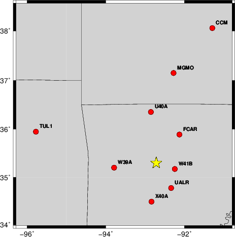
The focal mechanism was determined using broadband seismic waveforms. The location of the event and the and stations used for the waveform inversion are shown in the next figure.
|
|
|
|
The program wvfgrd96 was used with good traces observed at short distance to determine the focal mechanism, depth and seismic moment. This technique requires a high quality signal and well determined velocity model for the Green functions. To the extent that these are the quality data, this type of mechanism should be preferred over the radiation pattern technique which requires the separate step of defining the pressure and tension quadrants and the correct strike.
The observed and predicted traces are filtered using the following gsac commands:
hp c 0.02 n 3
lp c 0.10 n 3
The results of this grid search from 0.5 to 19 km depth are as follow:
           DEPTH  STK   DIP  RAKE   MW    FIT
WVFGRD96    0.5    90    65     0   3.94 0.9013
WVFGRD96    1.0    85    60   -10   3.98 0.9353
WVFGRD96    2.0    85    70   -20   4.00 0.9777
WVFGRD96    3.0    85    70   -20   4.01 0.9525
WVFGRD96    4.0    85    75   -15   4.01 0.9103
WVFGRD96    5.0    90    80   -15   4.01 0.8679
WVFGRD96    6.0   270    85    15   4.01 0.8343
WVFGRD96    7.0   270    75    10   4.02 0.8204
WVFGRD96    8.0   270    75    10   4.03 0.8067
WVFGRD96    9.0   270    75    10   4.03 0.7949
WVFGRD96   10.0   270    75    15   4.05 0.7845
WVFGRD96   11.0   270    75    15   4.05 0.7712
WVFGRD96   12.0   270    75    15   4.06 0.7581
WVFGRD96   13.0   270    75    10   4.07 0.7469
WVFGRD96   14.0   270    75    10   4.07 0.7360
WVFGRD96   15.0   270    75    10   4.08 0.7269
WVFGRD96   16.0   270    75    10   4.08 0.7185
WVFGRD96   17.0   270    75    10   4.09 0.7094
WVFGRD96   18.0   270    75    10   4.10 0.7012
WVFGRD96   19.0   270    75    10   4.11 0.6938
WVFGRD96   20.0   270    70    10   4.12 0.6856
WVFGRD96   21.0   270    70    10   4.12 0.6764
WVFGRD96   22.0   270    70    10   4.13 0.6707
WVFGRD96   23.0   270    70    10   4.13 0.6662
WVFGRD96   24.0   270    75    10   4.14 0.6614
WVFGRD96   25.0   270    80    15   4.14 0.6646
WVFGRD96   26.0   270    75     5   4.14 0.6683
WVFGRD96   27.0   270    75     5   4.15 0.6718
WVFGRD96   28.0   270    80    15   4.16 0.6759
WVFGRD96   29.0   265    70   -10   4.16 0.6814
WVFGRD96   30.0   265    70   -10   4.17 0.6879
WVFGRD96   31.0   265    70   -10   4.17 0.6916
WVFGRD96   32.0   265    70   -10   4.18 0.6940
WVFGRD96   33.0   265    70   -10   4.18 0.6934
WVFGRD96   34.0   265    70   -10   4.19 0.6931
WVFGRD96   35.0   265    70   -10   4.20 0.6915
WVFGRD96   36.0   265    70   -10   4.21 0.6886
WVFGRD96   37.0   270    75     5   4.22 0.6854
WVFGRD96   38.0   265    70    -5   4.24 0.6835
WVFGRD96   39.0   265    70    -5   4.25 0.6809
WVFGRD96   40.0   265    65   -10   4.29 0.6794
WVFGRD96   41.0   265    65   -10   4.30 0.6732
WVFGRD96   42.0   265    65   -10   4.31 0.6668
WVFGRD96   43.0   265    65   -10   4.32 0.6602
WVFGRD96   44.0   265    65   -10   4.32 0.6526
WVFGRD96   45.0   265    65   -10   4.33 0.6457
WVFGRD96   46.0   265    65   -10   4.34 0.6385
WVFGRD96   47.0   265    65   -10   4.35 0.6323
WVFGRD96   48.0   265    65   -10   4.35 0.6263
WVFGRD96   49.0   265    65   -10   4.36 0.6220
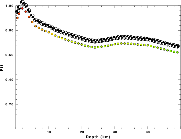
The best solution is
WVFGRD96 2.0 85 70 -20 4.00 0.9777
The mechanism correspond to the best fit is
|
|
|
The best fit as a function of depth is given in the following figure:
|
|
|
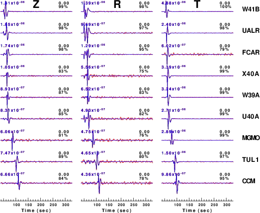
The comparison of the observed and predicted waveforms is given in the next figure. The red traces are the observed and the blue are the predicted. Each observed-predicted component is plotted to the same scale and peak amplitudes are indicated by the numbers to the left of each trace. A pair of numbers is given in black at the right of each predicted traces. The upper number it the time shift required for maximum correlation between the observed and predicted traces. This time shift is required because the synthetics are not computed at exactly the same distance as the observed and because the velocity model used in the predictions may not be perfect. A positive time shift indicates that the prediction is too fast and should be delayed to match the observed trace (shift to the right in this figure). A negative value indicates that the prediction is too slow. The lower number gives the percentage of variance reduction to characterize the individual goodness of fit (100% indicates a perfect fit).
The bandpass filter used in the processing and for the display was
hp c 0.02 n 3
lp c 0.10 n 3
|
|
|
|
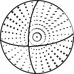
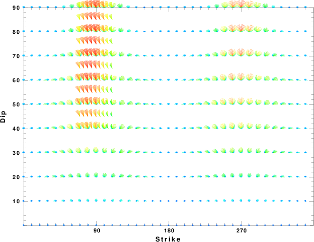
| Focal mechanism sensitivity at the preferred depth. The red color indicates a very good fit to thewavefroms. Each solution is plotted as a vector at a given value of strike and dip with the angle of the vector representing the rake angle, measured, with respect to the upward vertical (N) in the figure. |
A check on the assumed source location is possible by looking at the time shifts between the observed and predicted traces. The time shifts for waveform matching arise for several reasons:
Time_shift = A + B cos Azimuth + C Sin Azimuth
The time shifts for this inversion lead to the next figure:
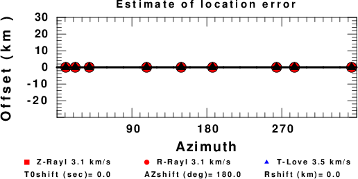
The derived shift in origin time and epicentral coordinates are given at the bottom of the figure.
The CUS model used for the waveform synthetic seismograms and for the surface wave eigenfunctions and dispersion is as follows:
MODEL.01
CUS Model with Q from simple gamma values
ISOTROPIC
KGS
FLAT EARTH
1-D
CONSTANT VELOCITY
LINE08
LINE09
LINE10
LINE11
  H(KM) VP(KM/S) VS(KM/S) RHO(GM/CC)   QP   QS  ETAP  ETAS  FREFP  FREFS
  1.0000  5.0000  2.8900  2.5000 0.172E-02 0.387E-02 0.00  0.00  1.00  1.00
  9.0000  6.1000  3.5200  2.7300 0.160E-02 0.363E-02 0.00  0.00  1.00  1.00
 10.0000  6.4000  3.7000  2.8200 0.149E-02 0.336E-02 0.00  0.00  1.00  1.00
 20.0000  6.7000  3.8700  2.9020 0.000E-04 0.000E-04 0.00  0.00  1.00  1.00
  0.0000  8.1500  4.7000  3.3640 0.194E-02 0.431E-02 0.00  0.00  1.00  1.00
Here we tabulate the reasons for not using certain digital data sets
The following stations did not have a valid response files: