Computer Programs in Seismology Tutorial

Ambient noise cross-correlation

Introduction

At the request of one user, this tutorial provides current scripts on the cross correlation of gound noise for the purpose of determining an interstation Green's function.

The complete package is contained in the archive noise.tgz which is 46 megabytes in size.

   NOISE
   |-- DATA
   |   -- 2010
   |       |-- 245
   |       |   |-- Q37ABHE
   |       |   |-- Q37ABHN
   |       |   |-- Q37ABHZ
   |       |   |-- R34ABHE
   |       |   |-- R34ABHN
   |       |   `-- R34ABHZ
   |       |-- 246
   |       |-- 247
   |       |-- 248
   |       |-- 249
   |       |-- 250
   |       |-- 251
   |       |-- 252
   |       |-- 253
   |       |-- 254
   |       |-- 255
   |       |-- 256
   |       |-- 257
   |       |-- 258
   |       |-- 259
   |       |-- 260
   |       |-- 261
   |       |-- 262
   |       |-- 263
   |       |-- 264
   |       |-- 265
   |       |-- 266
   |       |-- 267
   |       `-- 268
   |           |-- Q37ABHE
   |           |-- Q37ABHN
   |           |-- Q37ABHZ
   |           |-- R34ABHE
   |           |-- R34ABHN
   |           `-- R34ABHZ
   |-- DOCLEANUP
   |-- DOCONVERT
   |-- DOCORR
   |-- DOITALL
   |-- DOSTACK
   `-- bin
       -- DOPAIRDIST

This data set consists of 24 days of the Transportable Array stations Q37A and R34A together with processin scripts.

After modifying the scripts (see the discussion in the next section), the scripts are run in the following order:

DOCONVERT
DOITALL
DOSTACK

After the run there will be two new directories created: CROSS and STACK. The directory CROSS contains the cross-correlations for each day, e.g.,

CROSS/2010/268:
2010.268.Q37ABHRR34ABHR.cor  2010.268.Q37ABHTR34ABHT.rev
2010.268.Q37ABHRR34ABHR.rev  2010.268.Q37ABHZR34ABHZ.cor
2010.268.Q37ABHTR34ABHT.cor  2010.268.Q37ABHZR34ABHZ.rev

and the directory STACK will contain

Q37ABHRR34ABHR.WSTK  Q37ABHTR34ABHT.WSTK  Q37ABHZR34ABHZ.WSTK

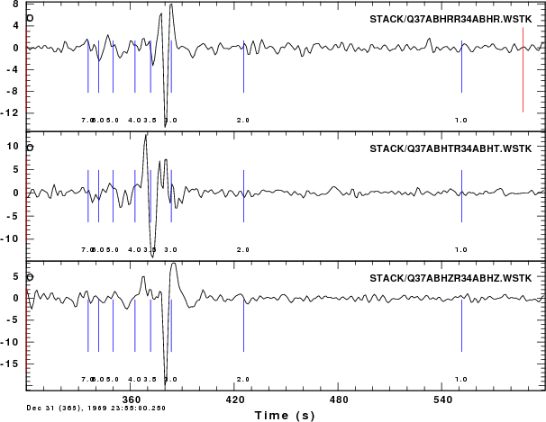
A plot of the 24 day stack of the cross-corelation (.cor) and reversed cross-correlation (.rev) is performed using the gsac commands

GSAC> r STACK/*
GSAC> xlim o o 300
GSAC> markt on
GSAC> p

plot of stack
The markt command indicates the group velocity. As can bee seen the Rayleigh wave is well developed on the R and Z components and the Love wave is well defined on the T component of the 24 day stack.

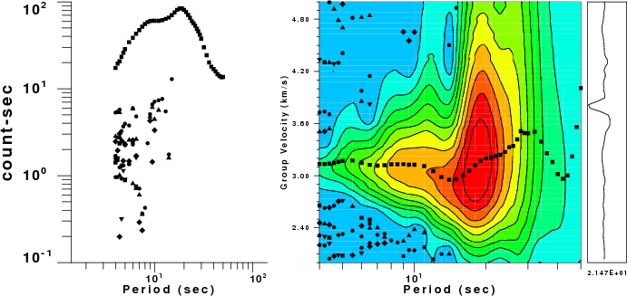
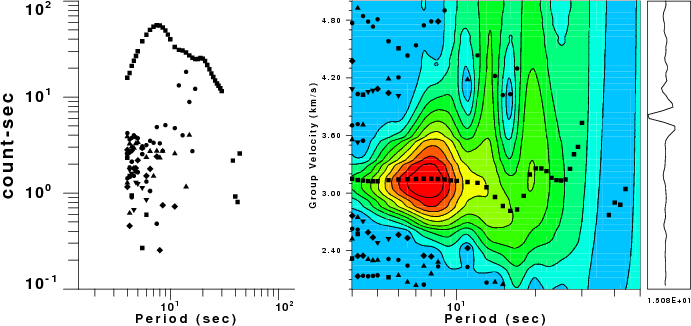
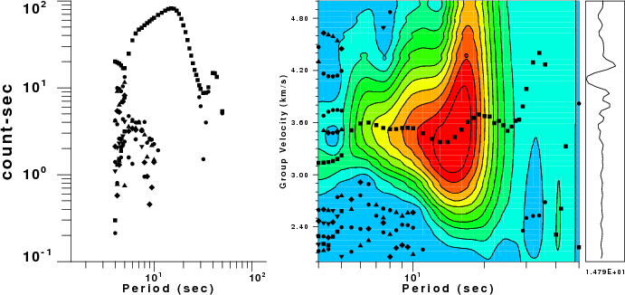
The group velocities are picked using the interactive program do_mft (which calls the program sacmft96 to do the processing). The plots resulting from sacmft96 are as follow:

Z

R

T

Scripts

Read the scripts carefully. If necessary purchase a book on BASH shell programming.

DOCONVERT - This script uses the Computer Programs in Seismology saccvt to ensure that the Sac files are in the proper binary format for you computer. If you create the Sac files on your computer, you will not require this

DOITALL - this script processes all data for the current year.

DOCORR - this script performs the cross-correlation, creates the directory CROSS, CROSS/YEAR and CROSS/YEAR/DAY

THIS SCRIPT MUST BE EDITED BEFORE YOU APPLY THIS TO YOUR DATA SETS. You must change the FREQLIMITS=, NPTSMIN and BASE entries for the following reason: to keep the size of this example small (and at 46 megabytes it is not small), I resamples the BH data to 1 sample/percond. This means that there is no signal at frequenices greater than 0.5 Hz, thus you must chang ehte FREQLIMTS parameter

NPTSMIN is used to check that I have approximately one day of data. At 1 sample per second, I there are 86400 seconds per day. Since I am getting these data from an archive, I will permit the data so start later than 0000 and to end before 235959. If you use 10 sample per second data, then this parameter should be TEN times larger.

BASE points to the location of the DATA files, e..g, ${BASE}/DATA has the entries above.

Note that the current code assumes that the files are BH (CMPZ, OCOMP and COMP parameters)

DOSTACK - this script stacks the cross-correlations and places them in the subdirectory STACK

Caution

Once you get the empirical Green's functions, you must then decide what the dispersion actually is. This requires practice since you must select a Gaussian filter parameter. I recommend starting with a reasonable estimate of the velocity model, making synthetics for the distances expected, and then selecting a Gaussial filter parmaeter (alpha) than best reproduces the known group velocities from the synthetic computations (modifiy the Surface-Wave Synthetics and Group Velocity Determination tutorial)

This exercise will also assist you in defining the period range that you can believe. You can only believe the long period estimates when you are are large distances.

Introduction

Contents:

Scripts

Caution