Computer Programs in Seismology Tutorial

Introduction

This tutorial considers wave propagation in water layers from 1.0 to 5.0km thick in order to assist the interpretation of OBS data. The ocean model is based on the AK135-F model developed at the Australian National University. The model was truncated to consist of just the water layer, crust and upper mantle and then converted to the MODEL96 format of Computer Programs in Seismology (CPS). The Q_κ and Q_μ were converted to Q_S using the relations Q^-1_P = L Q^-1_μ + (1 -L) Q^-1_κ and Q_S = Q_μ where L = (4/3)(V_P / V_S)² (Ben-Menahem and Singh, 10.03; Dahlen and Tromp, 9.59 and 9.60).

Thus the AK135F_AVG entry

Spherical average structure
    Depth    density  P vel    S vel    Q kappa     Q mu
      km      Mg/km3   km/s     km/s
     0.00    1.0200   1.4500   0.0000  57822.00     0.00
     3.00    1.0200   1.4500   0.0000  57822.00     0.00
     3.00    2.0000   1.6500   1.0000    163.35    80.00
     3.30    2.0000   1.6500   1.0000    163.35    80.00
     3.30    2.6000   5.8000   3.2000    1478.30  599.99
     10.00   2.6000   5.8000   3.2000    1478.30  599.99
     10.00   2.9200   6.8000   3.9000    1368.02  599.99
     18.00   2.9200   6.8000   3.9000    1368.02  599.99
     18.00   3.6410   8.0355   4.4839    950.50   394.62
     43.00   3.5801   8.0379   4.4856    972.77   403.93
     80.00   3.5020   8.0400   4.4800   1008.71   417.59
     80.00   3.5020   8.0450   4.4900    182.03    75.60
     120.00  3.4268   8.0505   4.5000    182.57    76.06
     120.00  3.4268   8.0505   4.5000    182.57    76.06
     165.00  3.3711   8.1750   4.5090    188.72    76.55
     210.00  3.3243   8.3007   4.5184    200.97    79.40
     210.00  3.3243   8.3007   4.5184    338.47   133.72
     260.00  3.3663   8.4822   4.6094    346.37   136.38
     310.00  3.4110   8.6650   4.6964    355.85   139.38

becomes

MODEL.01
AK135-F model converted to layers
ISOTROPIC
KGS
SPHERICAL EARTH
1-D
CONSTANT VELOCITY
LINE08
LINE09
LINE10
LINE11
 H(KM) VP(KM/S) VS(KM/S) RHO(GM/CC)   QP      QS ETAP ETAS FREFP FREFS
 3.000  1.450    0.000    1.020     0.000     0.000 0 0 1 1
 0.300  1.650    1.000    2.000   108.161    80.000 0 0 1 1
 6.700  5.800    3.200    2.600   927.336   599.990 0 0 1 1
 8.000  6.800    3.900    2.920   876.141   599.990 0 0 1 1
25.000  8.037    4.485    3.611   606.789   399.275 0 0 1 1
37.000  8.039    4.483    3.541   624.909   410.760 0 0 1 1
40.000  8.048    4.495    3.464   115.086    75.830 0 0 1 1
45.000  8.113    4.504    3.399   116.831    76.305 0 0 1 1
45.000  8.238    4.514    3.348   121.781    77.975 0 0 1 1
50.000  8.391    4.564    3.345   213.266   135.050 0 0 1 1
50.000  8.574    4.653    3.389   218.446   137.880 0 0 1 1
50.000  8.756    4.740    3.434   224.376   141.070 0 0 1 1
50.000  8.956    4.940    3.434   224.376   141.070 0 0 1 1

after replacing gradients by the average velocity (even though I should have used the average slowness to preserve vertical travel time).

This is just a test model.

In the examples developed below the models will be given with names like OCEAN_4.0.mod where the 4.0 indicates that the water layer is 4.0km thick instead of the original 3.0km. The examples will consider wave propagation with water layer thicknesses of 1.0, 2.0, 3.0, 4.0 and 5.0km.

Test scripts

Download the script OCEAN1.tgz and unpack it using the command

gunzip -c OCEAN1.tgz | tar xvf -
cd OCEAN1

You will see two directories. OCEAN_SW is for the surface wave study and OCEAN_WK is for the generation of a complete seismogram.

ls -F
OCEAN_SW/	OCEAN_WK/

Surface Wave

cd OCEAN_SW
DOITSW

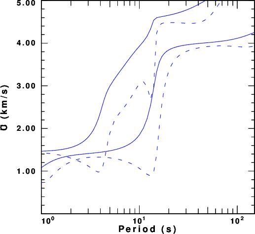
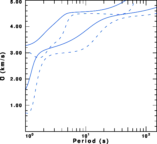
The purpose of this section is to compute the theoretical fundamental and first higher mode dispersion for Love and Rayleigh waves in each of the models. The computations and results will be in the sub-directories with names such as swDIR_5.0. The result will be the eigenfunction files slegn96.egn and sregn96.egn which are used by the program sdpegn96 to plot the dispersion. The shell script DOITSW performs the computations and creates the plots, which will be a superposition of the phase velocity (solid curve) and group velocities (dashed curve). The DOITSW assigns a different color to each depth from red at 1.0 to blue at 5.0 km. The individual plots in each sub-directory are named R.PLT and L.PLT. At the top level there are ALLL.PLT and ALLR.PLT.

For a water thickness of 5.0km, the dispersion plots are shown in the next figure.

Love wave fundamental and first higher mode

Rayleigh wave fundamental and first higher mode

The composite plot of all water depths is a little busy,

Composite Love wave fundamental and first higher mode. Orange=1.0km, blue=5.0km

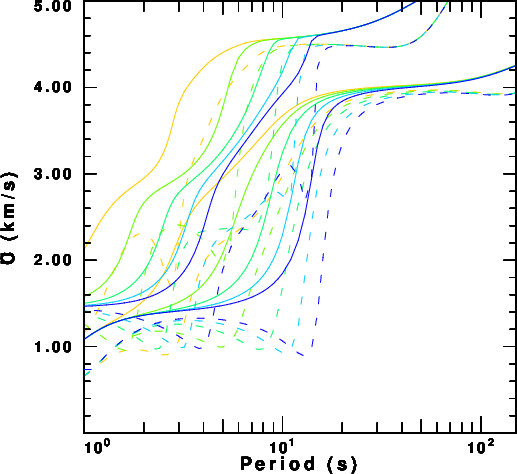
Composite Rayleigh wave fundamental and first higher mode. Orange=1.0km, blue=5.0km

This figure demonstrates two things. First all of the Love wave plots are the same since the Love wave is not affected by the surface water layer. Second the Rayleigh wave dispersion is very sensitive to the thickness of the water layer.

Suggestion

The model used is generic. It consists of a water layer, a sediment layer and a two layer crust. One might perturb the model to see the effect of the sediment thickness on the dispersion. It seems as if more can be learned about structure from an observation of the Love wave than from the Rayleigh wave.

Complete synthetics

After completing the surface wave computation, since we will use the eigenfunctions later when analyzing the dispersion using do_mft, enter the following command in the OCEAN_WK directory.

DOITWK

This script will create a sub-directory for each source depth. The computations and results will be in the sub-directories with names such as wkDIR_5.0. In order to make synthetics that can be used for interpretation of ambient noise from OBS seismometers on the sea bottom and, at the same time, account for efficient computation, the source is placed at a depth of 100m (0.1km) beneath the water-solid boundary and the receiver at a depth of 50m (0.05km) beneath the boundary. At long periods, this slight shift from a value of 0.0 will not affect the synthetics. Note: To obtain the Green's functions for a pressure field in the water, the receiver should be slightly above the boundary in the water.

The script will compute all Green's functions, but to understand the results of ambient noise analysis, the cross-correlation and stacking of the Z components (ZZ) will theoretically be the ZVF (vertical component observation due to a vertical force) Green's function, although the amplitude spectrum will be different. Part of this signal will be the Rayleigh wave. If ambient noise is obtained from the great circle path radial components (RR), RHF (radial due to horizontal force) is the Green's functions to consider, and finally THF will be appropriate for the TT cross-correlation. The purpose of these synthetics is to see what group and phase velocities may be obtained from the ambient noise results.

The script DOITWK will compute synthetics at distances of 100, 200, 300, 400 and 500km. As an example the next figure compares the ZVF, RHF and THF Green's functions at a distance of 500 km.

The next figure displays a record section of the THF and ZVF Green's functions for a water thickness of 5.0km.

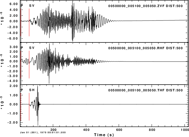
ZVF, RHF and THF Green's functions at a distance of 500km

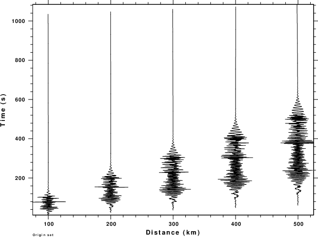
ZVF record section

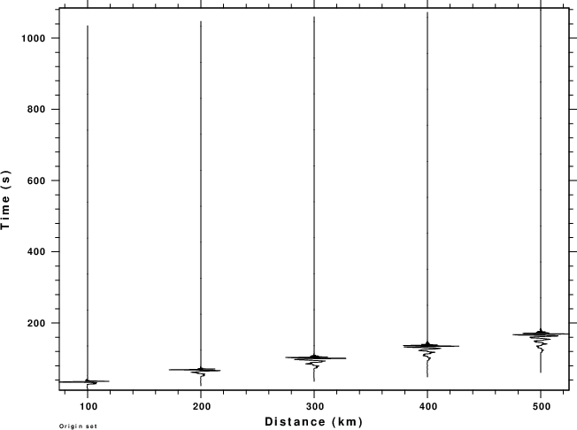
THF record section

Finally consider the THF and RVF Greens functions at a distance of 500km for different source depths.

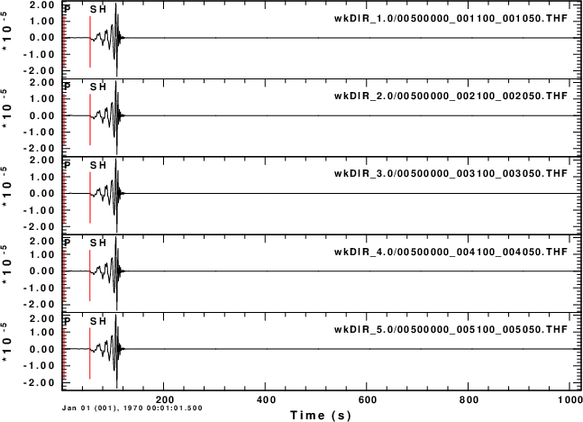
THF at 500km for source depths of 1.1, 2.1, ..., 5.1km

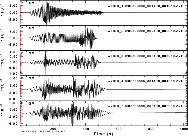
ZVF at 500km for source depths of 1.1, 2.1, ..., 5.1km

do_mft analysis

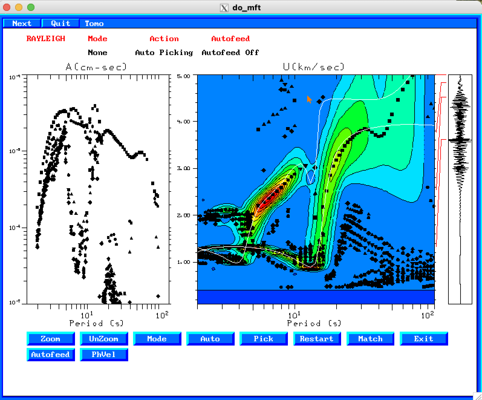
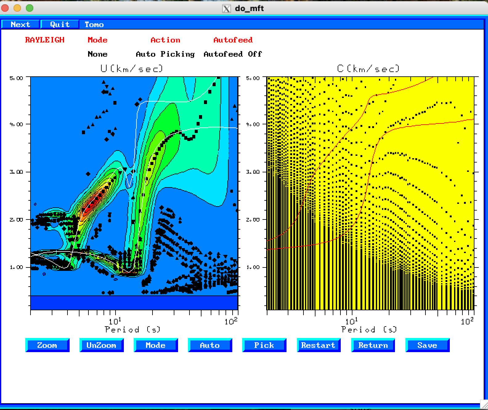
A use of the ambient noise empirical Green's functions is to determine group and phase velocity. The do_mft applies a multiple filter analysis to the seismograms. If shell scripts MFTDOOVERLAY and PHVDOOVERLAY have been created, then it is possible to overlay the theoretical model curves onto the dispersion estimate using the seismogram. When working with real data, this feature is used to determine an acceptable range of good observations. In this case with synthetics, this overlay permits one to understand the effects of the model on the determination of these velocities.

The next set of figures are screenshots of a set of do_mft windows. Comments will be placed at the bottom of each figure. In this example, the water is 5.0km deep, and we consider two separate runs - one for the ZVF traces and the other for the THF traces. The ZVF will be processed in detail at first, and just the important plots for the THF Green's functions will be displayed.

To keep the number of figures small, I will just indicate what "button" to press on each page. We will start with the ZVF synthetics.

cd wkDIR_5.0
do_mft -G -IG -T *ZVF

For assistance with this command just enter do_mft -h. the program is a GUI editor for the work done by the programs sacmft96 and sacmat96. The -G flag indicates that the name of the picked dispersion will have a .dsp or .phv appended to the file name for easier identification later. The -IG flag tells the program that the waveforms is an ambient noise Green's function of the type ZZ, RR or TT, and that the phase velocity should account for a π/4 phase shift of the source. Finally the -T flag indicates that the program should invoke the script MFTDOOVERLAY or PHVDOOVERLAY which is in the users PATH. These programs can be hand tailored to plot theoretical dispersion onto the observed seismogram dispersion. For this example, just the theoretical curves are overlain. I have more complicated scripts for North America which overlay theoretical curves for selected models and also the results of continental tomography.

Here are the steps taken to obtain the figures.

• Page 1 - Select a trace by clicking on the box. 005000000_005100_005050.ZVF is selected
• Page 2 - Click on "Unit" and select "Counts". For ambient noise empirical Green's functions. For these synthetics the actual units are cm/s. Then click on "Do MFT" at the top.
• Page 3 - Click on "Type: until Rayleigh appears since this is Z component observations.
  Click on "Vmin" to select the power "0.10" and then "1.0". This defines the minimum velocity of the plot to be 0.1 km/s.
  The "Alpha" parameter controls the Gaussian filter. A larger value has better frequency domain resolution but less time domain resolution because of the uncertainty principle. You might try different values to find the one that permits you to obtain the group and phase velocity.
  Click on "Do MFT".
• Page 4 - This is the interactive selection of dispersion values. To use a rubber band pick, click on "Auto" and then select the "Mode". Notice the "Tomo" button. Click on that and the MFTDOOVERLAY will be run and the dispersion plot redrawn. The result is
  
  The white curves on the plot are the theoretical values for the 5.0km model that were computed in OCEAN_SW. Note that Green's function has a large amplitude higher mode. Also note that the relative amplitudes displayed will be different for real data since the underlying amplitude spectrum of the noise will be different.
  Click on "PhVel"
• Page 5 - The region to the right is the phase velocity display while the figure on the left duplicates the group velocity display. the group velocities cannot be picked on this page, but are shown to indicate regions of large amplitude. At each period, the filtered trace is examined for the maximum amplitude of its envelope (used to determine the group velocity on Page 4). At this point the instantaneous phase is determined. The phase velocity is then computed for multiple values of 2π radian phase shifts (this is always an ambiguity in phase determination). If is up to the user to select the correct branch for the phase velocity.
  Click on "Tomo". this calls the script PHVOOVERLAY which plots the theoretical here as red curves. We see that it is very difficult to get the phase velocity using this technique in this case.
  The result is the picture
  

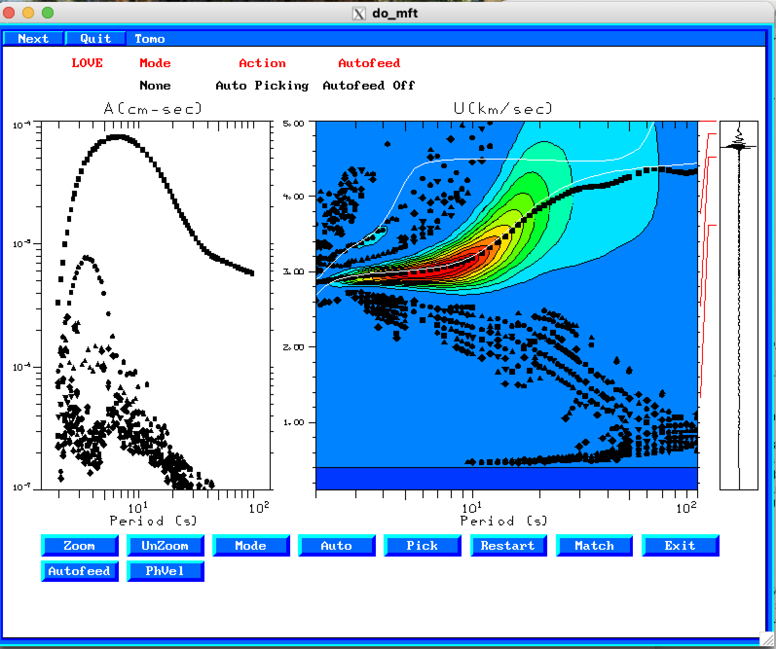
If we examine the THF Green's function which is related to the TT analysis, we obtain the following two figures after entering

do_mft -G -IG -T *THF

and being sure to select "Love" for "Type" on Page 3.

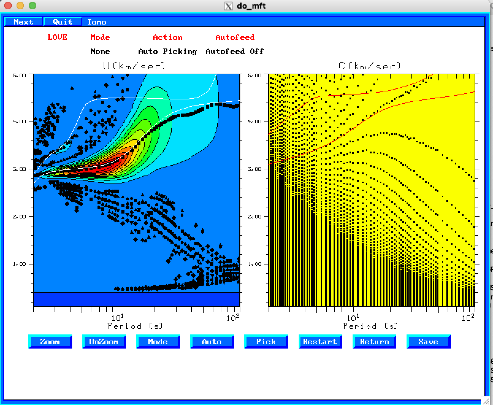In this case we actually get some good phase velocities except at very long periods.

Details on the scripts

the following links describe the processing scripts in detail.

• Scripts in OCEAN_SW
• Scripts in OCEAN_WK
• Conversion of CPS graphics to EPS and PNG