Sources generating elastic waves generate different amplitudes as a
function of takeoff angle and azimuth from the source. The convention
in seismology is to envision a sphere surrounding the source and the to
plot the signal amplitude on the sphere as the point where the ray from
the source to the receiver intersects the sphere. Such a plot can be
performed for any set of measurements, but typically one plots the
P-wave, SV-wave, SH-wave amplitude or the S-wave polarization at this
point. Rather than plotting this on an actual sphere, the upper
or lower half of this focal sphere is projected onto a piece of paper
tangent to the pole.
The convention of the takeoff angle is that a value of 0 represents a
ray going directly downward from the source into the earth, while a
value of 180 represents a ray propagating upward. The azimuth is
measured with respect to local north, with values of 0, 90, 180, and
270 representing north, east, south and west.
The lower hemisphere is defined by the combination of all azimuths and
takeoff angles from 0 to 90 degrees, while the upper hemisphere has
takeoff angles of 90 to 180 degrees.
The purpose of this section is to exercise the synthetics seismogram
programs to ensure that the conventions used for the Green's functions
and the focal mechanism are correct. We will accomplish this by making
wholespace synthetics (because of speed) using the programs mkmod96, hprep96, hwhole96, hpulse96,
fmech96 and
f96tosac .
We then use gsac to convert
the cylindrical coordinate traces to spherical radial, longitudinal and
latitudinal and to create the plot. We also use fmplot to plot the theoretical
amplitudes on the focal spheres, the program CAL to annotate the plot, plotnps to convert from CALPLOT
graphics to Encapsulated PostScript. We use the ImageMagick tool convert, available on LINUX,Cygwin
and OSX, to convert the Encapsulated PostScript to a Portable Network
Graphics (PNG) file. In addition we use the command gawk (locally called awk) as a
calculator.
The computer programs in seismology package creates Z - vertical, R - radial and T - transverse component synthetics for a cylindrical coordinate system, with the convention that Z is positive up, R is positive away from the source, and T is positive in a direction of increasing azimuth (using the convention above).
On a sphere we want the rotation to create the far-field P, SV and SH
waveforms, with P positive in a radial direction, SV positive as a
point on the ray moves in the direction of increasing takeoff angle,
and SH positive in the direction of increasing azimuth. The
necessary transformation is
R = Uradial = -UZ*COS(IO) + UR*SIN(IO)
T = Utheta  =  UZ*SIN(IO) + UR*COS(IO)
P = Uphi    = UT

where IO is the takeoff angle in radians ( angle in
radians = 3.1415926 * angle in degrees / 180)
The scripts used are as follow
Consider a double-couple focal mechanism with strike = 0, dip = 45 and
rake = 45 degrees. We will consider takeoff angles 0f 10, 30, 50 and 70
degrees for the lower hemisphere run and 110, 130, 150 and 170 degrees
for the upper hemisphere computations.
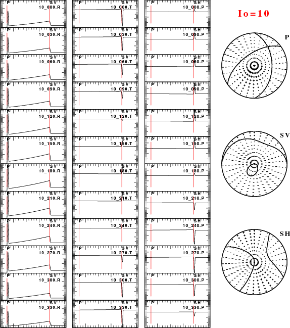
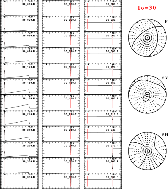
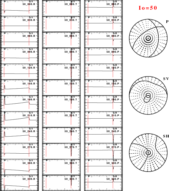
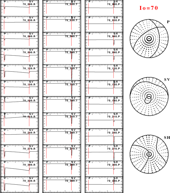
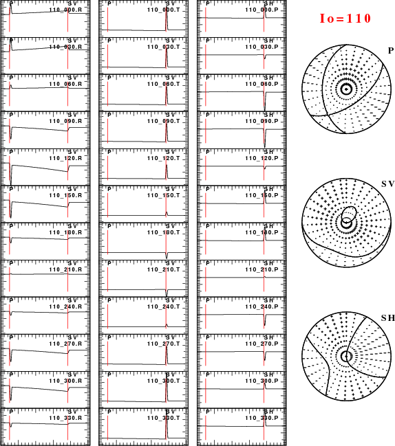
Each of the lines below present a figure with several components. There
are three columns of traces, arranged to highlight the far-field P (R),
SV (T) and SH (P) components of motion. Each plot is annotated as
IO_AZ_CMP, where IO is the takeoff angle in degrees AZ is the azimuth
in degrees and CMP is the trace component, e.g., R, T or P. For
each component the traces are plotted downward in order of increasing
azimuth. All traces of each component are plotted using the same
amplitude scale to be able to compare amplitudes. All traces represent
ground displacement.
To the right the P, SV and SH amplitudes are plotted on the focal
sphere. This plot shows an amplitude value of each of 30 azimuths and
10 takeoff angles, which are 10 degrees apart. The + and -
symbols indicate whether the amplitudes are positive or negative, and
the size of the symbol indicates relative amplitudes. The black curves
in these figures are nodal curves indicating the zero amplitude contour.
In the far-field, on can prove that the direction of vector S -motion
on the focal sphere is in the local direction of maximum increase of
P-wave amplitude on the sphere (gradient on the spherical surface).
When looking at the synthetics you will note some spikes as well as
some linear trends. The spikes are the far-field body-wave arrivals
which are superimposed on the near-field (linear ) trends. Focus on the
P-arrival on the Radial component, and the S arrivals on the SV and SH
components.