When ordering a SEED volume from IRIS, the contents will be both
the waveform as well as the data defining the station and instrument.
This latter part is called dataless SEED. Normally, I would unpack
the volume with the rdseed command
rdseed -f SEED_VOLUME -R -d -o 1
which will give the response in the RESP format, and dump the traces
in SAC format. It is also possible to get the network dataless SEED
files such as PBMOout.seed
RESP Files
If you desire to have the response file in the SEED RESP format
for use with the program evalresp, execute the command
rdseed -f PBMOout.seed -R
which then produces the RESP files with the naming convention
RESP.NETWORK.STATION.LOCATION.COMPONENT:
The RESP files provide the complete response as stages, starting with
ground motion, sensor, digitizer, through all digital filtering. This
file is a complete physical description of the response.
To use the RESP file to define the instrument response, the
utility program evalresp is used:
where STATION_NAME is the station code, COMPONENT_NAME is the
component. YEAR and DAY_OF_YEAR are used to get the response for a
given day, since the RESP file can provide the complete instrument
history of a station/component. FMIN, FMAX and NFREQ tell evalresp
to create tables of frequency-amplitude and frequency-phase with
NFREQ values between FMIN and FMAX. The argument of the -u
flag indicates the desired units for the table. If the argument is
DIS, the response will be COUNTS per METER input ground displacement.
If the argument is VEL, the response is COUNTS per METER/SEC input
ground velocity. If the argument is ACC, the response is COUNTS per
METER/SEC/SEC input ground acceleration.
For the sample dataless SEED given above, the command
The polezero files for seismic sensors created by rdseed from
the SEED volume, provides the transfer function from ground
displacement in units of METERS to COUNTS. For the BHZ
channel, the contents are
We can use gsac to present the amplitude spectra of the
responses:
gsac << EOF
#####
#       create an impulse with unit area
#####
fg impulse delta 0.05 npts 8192
w imp.sac
r imp.sac
ch KSTNM PBMO
ch KCMPNM BHZ
wh
#####
#       obtain the velocity sensitivity
#####
transfer from none to eval subtype AMP.NM.PBMO..BHZ PHASE.NM.PBMO..BHZ
w velcount.sac
fft
bg plt
color list red
psp fmin 0.01 fmax 20
plotnps -F7 -W10 -EPS -K < P001.PLT > respplot.eps
convert -trim respplot.eps respplt.png


#####
#       obtain the displacement sensitivity
#####
r imp.sac
transfer from none to polezero subtype \
           SAC_PZs_NM_PBMO_BHZ__2007.173.00.00.00.0000_99999.9999.24.60.60.99999
w discount.sac
fft
color list blue
psp fmin 0.01 fmax 20
plotnps -F7 -W10 -EPS -K < P002.PLT > pzplot.eps
convert -trim pzplot.eps pzplt.png
quit
EOF
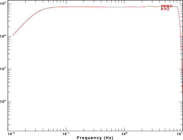
The amplitude response can be viewed
Velocity sensitivity in COUNTS/M/SEC using evalresp -u
'vel' output. Note that at high frequencies, the effect of the
FIR filters is seen.
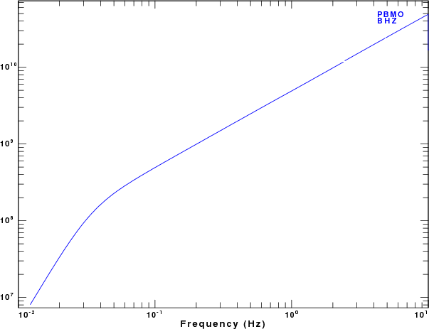
Displacement sensitivity in COUNTS/M using the polezero files.
Note that the polezero files do not include the effect of the FIR
filters. Also note that the Displacement and velocity sensitivity
values are identical for OMEGA ( 2 pi f ) = 1 radian/sec, or a
frequency of about 0.16 Hz.
Removing the response
Removing the instrument response must be done carefully because
real data will have noise and dividing by the low response at high or
low frequencies will enhance the noise. The safe way to do this is to
apply a bandpass filter as part of the deconvolution.
Consider the output due to an impulse in ground velocity, which is
created by the gsac commands:
r imp.sac
transfer from none to eval subtype AMP.NM.PBMO..BHZ PHASE.NM.PBMO..BHZ
w velcount.sac
This transfer function removes both the high and low frequencies, as
seen from the plot above.
If there is noise added to the recording that is not related to
the instrument, then removal of the instrument will enhance that
noise. To remove the instrument response, the following is a safe
procedure:
#####
#       define the frequency limits for deconvolution
#####
DELTA=`saclhdr -DELTA velcount.sac`
FHH=`echo $DELTA | awk '{print 0.50/$1}' `
FHL=`echo $DELTA | awk '{print 0.25/$1}' `


#####
#       now try a deconvolution with the FREQLIMITS
#####
gsac << EOF
r velcount.sac
transfer from eval subtype AMP.NM.PBMO..BHZ \
          PHASE.NM.PBMO..BHZ to none freqlimits 0.005 0.01  ${FHL} ${FHH}
w deconvelfl.sac
quit
EOF
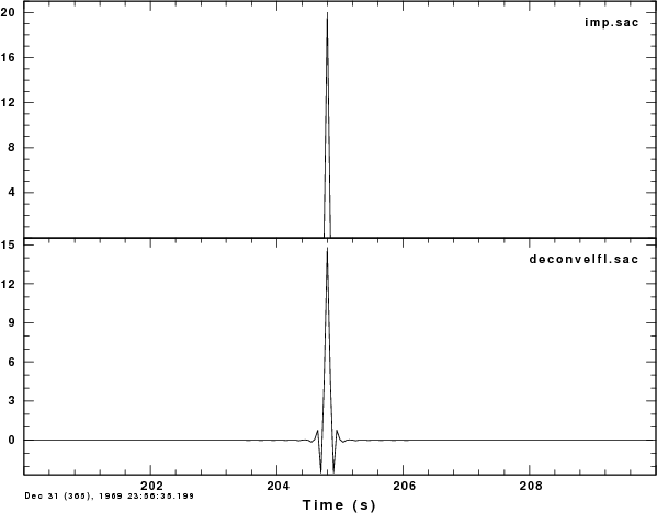
Note that this automatically adjusts for the sample rate (DELTA) to
compute the Nyquist frequency (FHH). the result will be a bandpass
filtered version of the desired ground motion:
Original (top) and deconvolved ground velocity
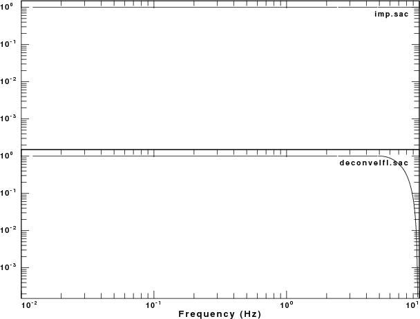
Original (top) and deconvolved ground velocity spectrum. Note
the bandpass filtering action.