Seismic Exploration Synthetics - Part I

Introduction

The synthetic seismogram code for Computer Programs in Seismology is designed to provide the medium response to a step in seismic moment for moment tensor source and a step force for point force sources. The source time function selection permits a rise time, to reflect the earthquake source duration, through the selection of triangular and parabolic pulses. These are discussed in Appenxid B of the Computer Program ins Seimology - Overview document ( PROGRAMS.330/DOC/OVERVIEW.pdf/cps330o.pdf). The use of the triangular and parabolic pulses have the benefit making clean looking synthetics to remove the noise caused by a sharp trunction at the Nyquist frequency.

To be able to use the Green's functions computed using the shortest duration source pulse to model large earthquakes, the gsac commands triangle, boxcar or trapezoid can be used to make the source pulse longer.

The programs used to convolve the source pulse are hpulse96, spulse96, gpulse96 and cpulse96 for use with the wave-number integration, modal superposition, generalized ray and asymptotic ray tracing synthetics. These codes specificy the source pulses with the following command line flags:

-p -l L Use a parabolic pulse of duration 4L dt, where dt is the sampling interval
-t -l N Use a trialgular pulse of duration 2N dt for N > 1 [ -p -L 1 is equivalent to -t -l 2 ]
-F rfile Use the pulse defined by the contents of the file rfile [See the subroutine pupud in the source code for the format ]
-i Use an impulse (e.g., true step source with zero rise-time. The pulse definitions description given here represent the derivative of the source time function).

In addition the user can specify the type of synthetic, -A for acceleration, -V for velocity and -D for displacement.

Recently, October 28, 2011) a user had problems with using the -F rfile to apply a Ricker wavelet. There may be a problem in the code, but one source may be the fact that the maximum of the Ricker wavelet occurs at some time after the initial point and there is no easy way to zero phase the pulse when making the synthetics. As a solution gsac now can convolve a waveform with a zero phase Ricker wavelet.

Before making synthetics, we should discuss source time functions for exploration. This is more convoluted than for the earthquake source problem, since the earthquake source time function must be step like to represent the permanent deformation due to an earthquake.

If we wish to model a simple explositon, a step in isotropic moment may be adequate, although some overshoot should be allowed according the Sharpe (1942) model [Sharpe, J. A., (1942). Production of elastic waves by explosion pressures, Geophysics 7, 144-154]. If we wish to model a weight drop, a simple step in force at the surface may not be adequate. Following Day et al (1983) [Day, S. M., N. Rimer and J. T. Cherry (1983). Surface waves from underground explosions with spall analysis of elastic and nonlinear source models, Bull. Seism.Am. 73, 247-264.], the applied force may be as in the next figure:

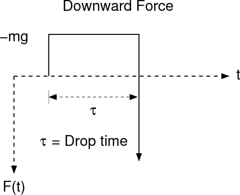
When the weight is released, there is a negative force applied to the ground at the weight supports. The weight falls because of gravity a time τ seconds, when it impacts the ground the source time function may be represented as

F(t) = -mg [ H(t) - H(t - τ) ] + mgτ δ (t-τ)

This relation assures that momentum is conserved. To see this phenomena, one must start recording at the instant the weight is released rather than at the time of impact. For high frequency seismograms, the waves generated by the impulsive point force will dominate the record.

To actually make a synthetic that looks like real observations, one must simulate the source, as duscussed above, and then place the record through a geophone, which outputs a voltage proportional to a high-pass filtered ground velocity. The geophone introduces a shape to the waveforms.

Download

Download the file ricker.tgz and unpack using the command

             gunzip -c ricker.tgz | tar xvf -
             cd RICKER

There will be a shell script DOFIT and two subdirectories, WK and SW. The wavenumber integration synthetics are in WK and the fundamental mode surface wave synthetics are in SW.

To make the synthetics,

            cd RICKER
            cd SW
            DOIT-sw
            cd ..
            DOIT-wk
            cd ..

            DOFIT  (script to make the plots below)

Sample Run

The DOIT-sw and DOIT-wk scripts differ only in the use of the synthetics seismogram programs. The annotated DOIT-wk script
is as follows:

#!/bin/bash

rm -fr ORIG RICKER

#####
# MODEL 1 , dr pujol, date 23 Aug 2011, from paper 
# "shear wave velocity profiling, at sites with high 
# freqeuncy stiffness contrasts: a comparison between 
# invasive and non-invasive methods", TABLE 1
#
# Create the model using mkmod96                              CREATE THE VELOCITY MODEL USING mkmod96
#####                                                         THIS IS COMMENTED SINCE THE MODEL IS GIVEN BELOW
#mkmod96 << EOF
#simple.mod
#Simple Crustal Model
#0
#0.0050 1.100 0.300 1.6 20 20 0 0 1 1
#000000 1.800 0.400 2.0 20 20 0 0 1 1
#EOF


cat > simple.mod << EOF
MODEL.01
Simple Crustal Model
ISOTROPIC
KGS
FLAT EARTH
1-D
CONSTANT VELOCITY
LINE08
LINE09
LINE10
LINE11
  H(KM) VP(KM/S) VS(KM/S) RHO(GM/CC)  QP   QS  ETAP  ETAS  FREFP  FREFS 
  0.0050  1.1000  0.3000  1.6000 20.0  20.0  0.00  0.00  1.00  1.00 
  0.0000  1.8000  0.4000  2.0000 20.0  20.0  0.00  0.00  1.00  1.00 
EOF

cat > dfile << EOF
0.002   0.0005  512     -0.05   0                           DEFINE THE DISTANCES, NUMBER OF POINTS AND SAMPLE INTERVAL
0.004   0.0005  512     -0.05   0                           THIS WAS ORIGINALLY 0.00025 FOR SAMPLING INTERVAL AND 1024
0.006   0.0005  512     -0.05   0                           POINTS.  THIS MAKES THE COMPUTATIONAL TIME SIGNIFICANTLY
0.008   0.0005  512     -0.05   0                           LONGER
0.01    0.0005  512     -0.05   0
0.012   0.0005  512     -0.05   0
0.014   0.0005  512     -0.05   0
0.016   0.0005  512     -0.05   0                           NOT THAT THE TIME SERIES DOES NOT START NOT AT 0 SEC BUT 0.05 SEC
0.018   0.0005  512     -0.05   0                           BEFORE THE ORIGIN TIME. THIS IS DOME SINCE THE USE OF THE SYMMETRIC RICKER
0.02    0.0005  512     -0.05   0                           WAVELET EXTENDS INTO NEGATIVE TIME AT SHORT DISTANCE
0.022   0.0005  512     -0.05   0
0.024   0.0005  512     -0.05   0
0.026   0.0005  512     -0.05   0
0.028   0.0005  512     -0.05   0
0.03    0.0005  512     -0.05   0
EOF

hprep96 -M simple.mod -d dfile -HS 0.002 -HR 0 -EXF
hspec96 > hspec96.out
hpulse96 -p -V -l 1  |  f96tosac -B                        GENERATE GROUND VELOCITY. USE THE parabolic pulse TO AVOID GIBB's EFFECTS

mkdir ORIG
mv *sac ORIG

#####
#    differentiate the point force synthetics
#    to simulate a delta function source 
#####
gsac << EOF
r ORIG/*VF.sac ORIG/*HF.sac
dif
w
q
EOF

#####
#  convolve with a Ricker wavelet
#####
mkdir RICKER
FREQ_RICKER=25
gsac << EOF
##### process the explosion sources                THE RICKER FILTERED TRACES ARE OF GROUND VELOCITY TO SIMULATE A GEOPHONE WITH
cd ORIG                                            NATURAL FREQUENCY LESS THAN 25 Hz.
r *.sac
ricker f ${FREQ_RICKER}
cd ../RICKER
w
q
EOF


#####
#   clean up
#####
rm -f dfile hspec96.dat hspec96.grn hspec96.out simple.mod

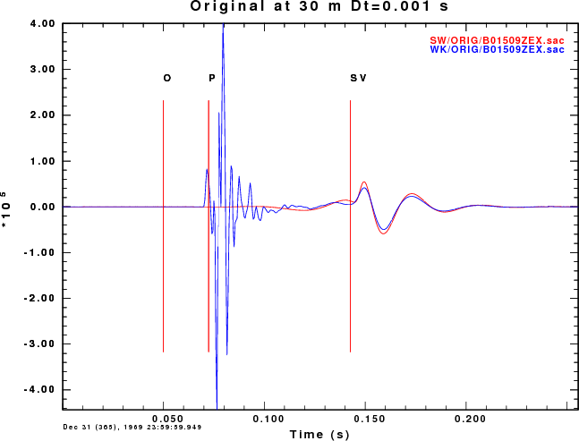
The first comparison is of the B01509ZEX.sac and B01511ZVF.SAC files from each technique the gsac command for the plot is

r SW/ORIG/B01509ZEX.sac WK/ORIG/B01509ZEX.sac
color list red blue
fileid name
ylim all
bg plt
title on l top s m text "Original at 30 m Dt=0.001 s"
p overlay on
plotnps -F7 -W10 -EPS -K < P001.PLT > t.eps ; gm convert -trim t.eps ZEX.over.o.png
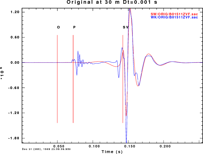
r SW/ORIG/B01511ZVF.sac  WK/ORIG/B01511ZVF.sac
p
plotnps -F7 -W10 -EPS -K < P002.PLT > t.eps ; gm convert -trim t.eps ZVF.over.o.png
q

The plots comparing the synthetics for the ZEX and ZVF Greens functions for the surface-wave SW (red) and wavenumber integration (blue). The difference between a fundamental mode synthetic and the complete solution are obvious. We also see that the high frequency generation of P waves is greater for the explosion source.

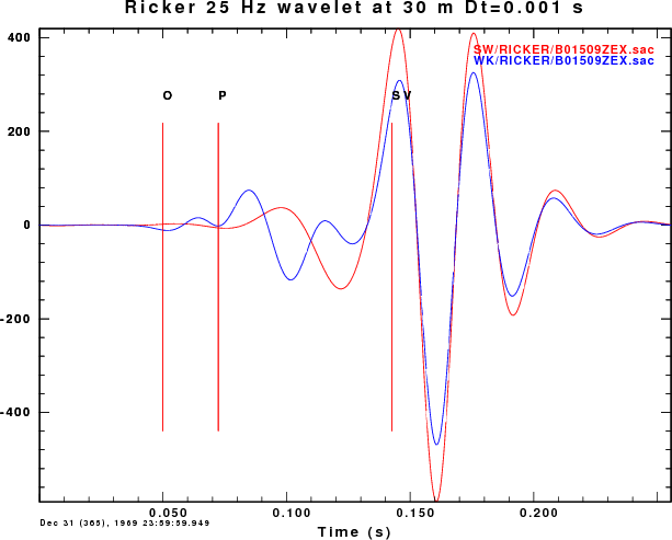
The next comparison is of the B01509ZEX.sac and B01511zvf.SAC files from each technique which have been convolved with the Ricker wavelet. The gsac command for the plot is


r SW/RICKER/B01509ZEX.sac WK/RICKER/B01509ZEX.sac
lh delta dist
color list red blue
fileid name
ylim all
bg plt
title on l top s m text "Ricker 25 Hz wavelet at 30 m Dt=0.001 s"
p overlay on
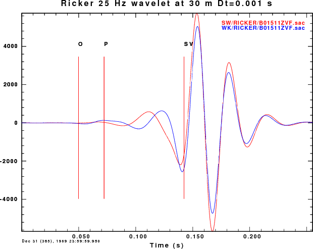
r SW/RICKER/B01511ZVF.sac  WK/RICKER/B01511ZVF.sac
p
q

The plots comparing the synthetics for the ZEX and ZVF Greens functions for the surface-wave SW (red) and wavenumber integration (blue)

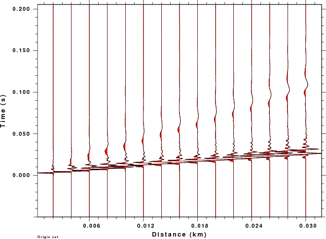
The final comparison provides record sections for the explosion source for the original and wavelet filtered traces are created using the gsac commands:

r WK/ORIG/*ZEX.sac
bg plt
prs shd pos color 2
r WK/RICKER/*ZEX.sac
prs 
q

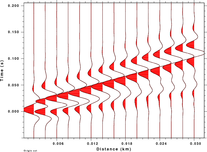
The plots resulting plots for the original traces and Ricker wavelets are given in the next plot:

Original Traces	Ricker Wavelet