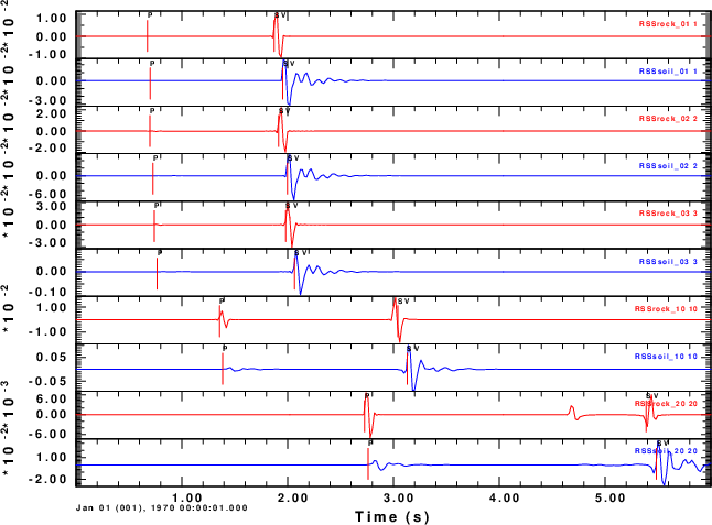
Comparison of the radial component traces for the Rock (red) and Soil (blue) traces as a function of epicentral distance.
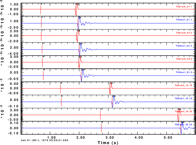
Comparison of the transverse component traces for the Rock (red) and Soil (blue) traces as a function of epicentral distance.
DOPLTPNG
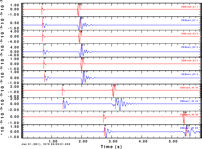
Comparison of the vertical component traces for the Rock (red) and Soil (blue) traces as a function of epicentral distance.
The arrival between P and S at 20 km on the rock trace is an artifact of the wavenumebr integration and can be controlled by effectively making the Δk smaller. The waveforms are simpler in appearance since we are3 essentially looking at the direct P and S rays from the source. The traces for the soil model show some reverberations.
The next step was to window the traces on the S wave, take the Fourier transform and then save the amplitude spectra.
At each distance a spectral ratio was obtained and the ration for each component were compared to the quarter-wavelength formula.
The plots for the five distances are as follow:
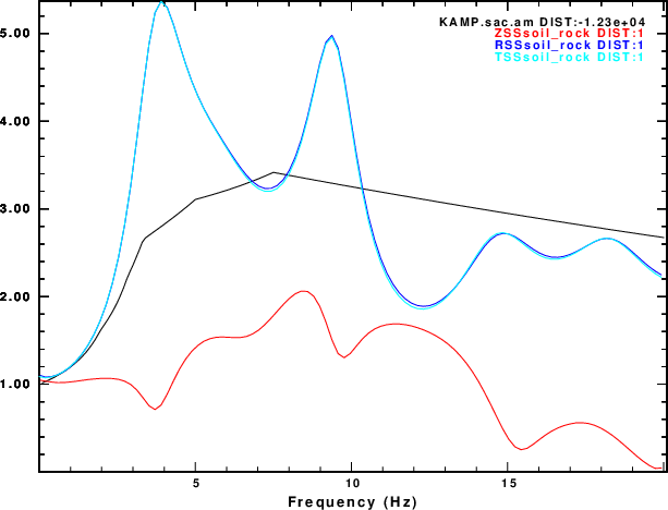 Site effect ratios at an epicentral distance of 1.0 km. |
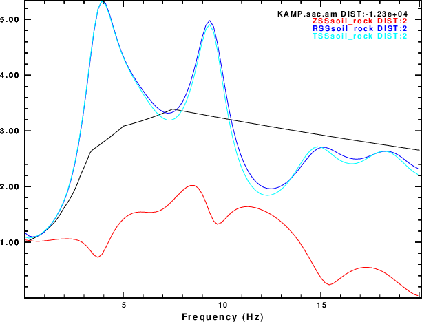 Site effect ratios at an epicentral distance of 2.0 km. |
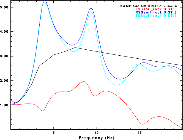 Site effect ratios at an epicentral distance of 3.0 km. |
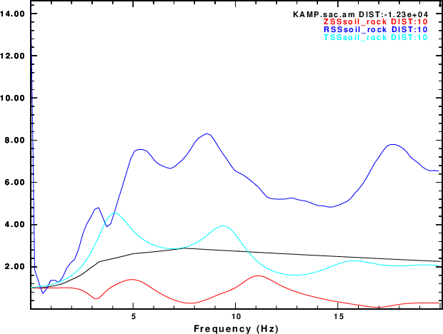 Site effect ratios at an epicentral distance of 10.0 km. |
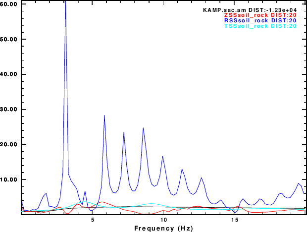 Site effect ratios at an epicentral distance of 20.0 km. |
The spectral ratios at 1, 2 and 3 km look very similar to the plane wave results. The quarter-wavelength formula seems to fit the horizontal R and T components.
At a distance of 10km the amplification on the radial component increases, while at 20 km, this amplification becomes very large, although the rations of the Z and T components seem to behave well.
DOPLTPNG
#!/bin/sh

for i
do
B=`basename $i .PLT`
plotnps -F7 -W10 -EPS -K < $i > t.eps
convert -trim t.eps -background white -alpha remove -alpha off ${B}.png
rm t.eps
done