Computer Programs in Seismology Tutorial

Surface wave inversion kernels - I

Changes

15 AUG 2013 - corrected error in the EXAMPLE_2/DOPLT. The maximum amplitude from the file love was use for the Rayleigh plots instead of the maximum amplitude ion the rayl file.
09 SEP 2013 - added EXAMPLE_3/DOPLTz to plot modified AK135 kernels as a function of depth rather than layer number

Introduction

Although the programs surf96 and joint96 have been available for a long time, access to the actual partial derivatives used in the inversion of surface-wave data has not been easily accessible unless one really read the programs. Many investigators would like access to these partials to better understand the inversion process. This tutorial and the new program srfker96 installed in PROGRAMS.330/VOLIV/src of the distribution provides the theory and the ability to get the information.

The detailed theory is given in surf.pdf. The discussion shows how the program surf96 procides the required partial derivatives, especially those for the group velocity partials which are obtained numerically and are thus not available from the eigenfunciton programs in PROGRAMS.330/VOLIII/src, e.g., sregn96 and slegn96.

The complete set of scripts for running the programs are given in DIST.tgz. After downloading, upack using the command:

gunzip -c DISP.tgz | tar xvf -

This will create the subdirectory SWKERNELS/DIST. cd SWKERNELS/DIST. There are three subdirectories: EXAMPLE_1 and EXAMPLE_2 which have the control files for the two examples in the next section, and Source. The subdirectory Source has three files: srfker96.f, tMakefile and tmpjsamat.f. The last two are used in the testing section. If you do not wish to upgrade the CPS package, you can just compile and run the srfker96.f with the following gfortran command:

gfortran -frecord-marker=4 srfker96.f -o srfker96

Use of srfker96

Example 1

The first example is in the subdirectory EXAMPLE_1. In this directory you will find the following files: sobs.d, CUS.mod and tdisp.d. The CUS.mod is a model file in the model96 format, the tdisp.d is a dispersion file, with fake entries. The only required features are the wave type, group velocity, mode and period entries. The sobs.d is the control file for the program surf96.

Given these files, run the following sequence of commands:

surf96 39
surf96 1
srfker96 > srfker96.txt
surf96 39

The surf96 39 cleans up temporaty files, surf96 1 computes the partials, and srfker96 provides the desired kernels. The control file sobs.d is

  4.99999989E-03  4.99999989E-03   0.0000000      4.99999989E-03   0.0000000 
    1    1    1    1    1    1    1    0    1    0
CUS.mod                  
tdisp.d

The velocity model CUS.mod is:

MODEL.01
CUS Model with Q from simple gamma values
ISOTROPIC
KGS
FLAT EARTH
1-D
CONSTANT VELOCITY
LINE08
LINE09
LINE10
LINE11
  H(KM) VP(KM/S) VS(KM/S) RHO(GM/CC)   QP   QS  ETAP  ETAS  FREFP  FREFS
  1.0000  5.0000  2.8900  2.5000 0.172E-02 0.387E-02 0.00  0.00  1.00  1.00 
  9.0000  6.1000  3.5200  2.7300 0.160E-02 0.363E-02 0.00  0.00  1.00  1.00 
 10.0000  6.4000  3.7000  2.8200 0.149E-02 0.336E-02 0.00  0.00  1.00  1.00 
 20.0000  6.7000  3.8700  2.9020 0.000E-04 0.000E-04 0.00  0.00  1.00  1.00 
  0.0000  8.1500  4.7000  3.3640 0.194E-02 0.431E-02 0.00  0.00  1.00  1.00

and the dispersion file tdisp.d is

SURF96 L U X   0     10.0000     4.0000     0.1000
SURF96 R U X   0     10.0000     4.0000     0.1000

and the output of srfker96 is srfker96.txt

___________________________________________________________________________________________
Elastic  Love wave:     Period=    10.000 Mode =    0 C=     3.697 U=     3.471
LAYER    THICK     dc/db      dU/db      dc/dh      dU/dh
    1     1.000  5.438E-02  9.366E-02 -5.011E-02 -7.176E-02
    2     9.000  5.469E-01  8.137E-01 -1.346E-02 -7.754E-03
    3    10.000  3.361E-01  2.380E-01 -4.711E-03  2.603E-03
    4    20.000  1.517E-01 -1.027E-01 -1.102E-03  2.980E-03
    5     0.000  5.138E-03 -1.944E-02  0.000E+00  0.000E+00
___________________________________________________________________________________________
Anelastic Love wave:     Period=    10.000 Mode =    0 C=     3.688 U=     3.466 GAMMA=  2.731E-04
LAYER    THICK     dc/db      dU/db      dc/dh      dU/dh     dc/dQbi    dU/dQbi    dg/dQbi
    1     1.000  5.422E-02  9.363E-02 -5.011E-02 -7.176E-02 -1.152E-01 -7.065E-02  3.613E-03
    2     9.000  5.454E-01  8.133E-01 -1.346E-02 -7.754E-03 -1.411E+00 -8.655E-01  4.425E-02
    3    10.000  3.353E-01  2.374E-01 -4.711E-03  2.603E-03 -9.116E-01 -5.591E-01  2.859E-02
    4    20.000  1.517E-01 -1.031E-01 -1.102E-03  2.980E-03 -4.304E-01 -2.640E-01  1.350E-02
    5     0.000  5.122E-03 -1.949E-02  0.000E+00  0.000E+00 -1.770E-02 -1.086E-02  5.551E-04
___________________________________________________________________________________________
Elastic  Rayleigh wave: Period=    10.000 Mode =    0 C=     3.341 U=     3.111
LAYER    THICK     dc/da      dc/db      dU/da      dU/db      dC/dh      dU/dh
    1     1.000  2.239E-02  2.732E-02  4.218E-02  4.471E-02 -4.678E-02 -6.223E-02
    2     9.000  8.043E-02  2.548E-01  6.769E-02  6.575E-01 -1.478E-02 -1.451E-02
    3    10.000  7.740E-03  3.729E-01 -1.278E-02  3.370E-01 -5.335E-03  5.341E-03
    4    20.000  6.406E-04  1.460E-01 -3.060E-03 -2.495E-01 -6.882E-04  3.490E-03
    5     0.000  7.467E-06  2.250E-03 -5.734E-05 -1.402E-02  0.000E+00  0.000E+00
___________________________________________________________________________________________
Anelastic Rayleigh wave: Period=    10.000 Mode =    0 C=     3.334 U=     3.107 GAMMA=  2.616E-04
LAYER    THICK     dc/da      dc/db      dU/da      dU/db      dc/dh      dU/dh     dc/dQai    dc/dQbi    dU/dQai    dU/dQbi    dg/dQai    dg/dQbi
    1     1.000  2.237E-02  2.725E-02  4.219E-02  4.469E-02 -4.678E-02 -6.223E-02 -8.207E-02 -5.788E-02 -5.077E-02 -3.581E-02  3.152E-03  2.223E-03
    2     9.000  8.033E-02  2.541E-01  6.762E-02  6.576E-01 -1.478E-02 -1.451E-02 -3.596E-01 -6.574E-01 -2.225E-01 -4.067E-01  1.381E-02  2.525E-02
    3    10.000  7.731E-03  3.720E-01 -1.282E-02  3.365E-01 -5.335E-03  5.341E-03 -3.630E-02 -1.011E+00 -2.246E-02 -6.257E-01  1.394E-03  3.884E-02
    4    20.000  6.406E-04  1.460E-01 -3.065E-03 -2.500E-01 -6.882E-04  3.490E-03 -3.146E-03 -4.140E-01 -1.946E-03 -2.561E-01  1.208E-04  1.590E-02
    5     0.000  7.457E-06  2.243E-03 -5.744E-05 -1.405E-02  0.000E+00  0.000E+00 -4.461E-05 -7.750E-03 -2.760E-05 -4.795E-03  1.713E-06  2.976E-04
___________________________________________________________________________________________

Note that there are entries for each line of the dispersion file which contain listings of the partial derivatives without and with the effects of Q.

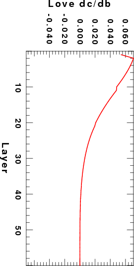
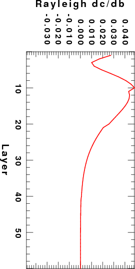
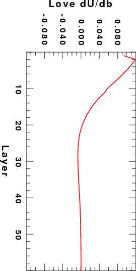
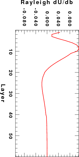
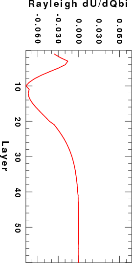
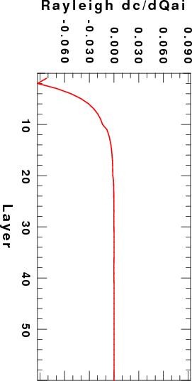
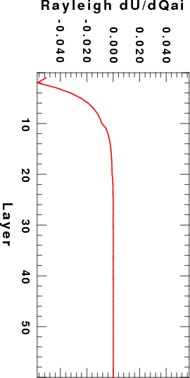
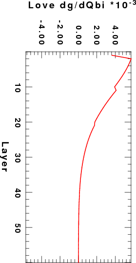
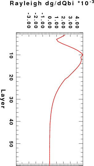
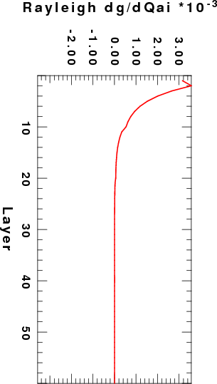
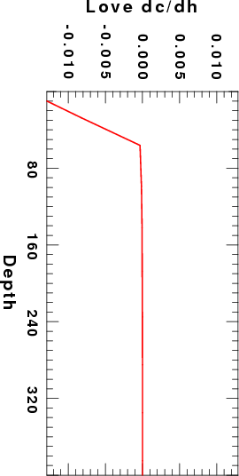
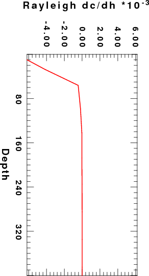
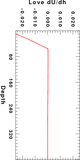
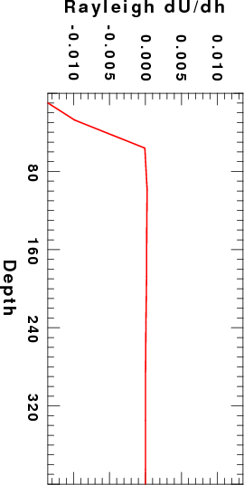
Example 2 - Kernels as a function of layer number

The second example uses the same velocity model as the CUS.mod, but now splitting each layer into 1 km sup-layers, so that the partial derivatives can be plotted. The data set is in the subdirectory EXAMPLE_2. The only difference is that now sobs.d is

  4.99999989E-03  4.99999989E-03   0.0000000      4.99999989E-03   0.0000000 
    1    1    1    1    1    1    1    0    1    0
dCUS.mod                  
tdisp.d

The same commands are run, and the output is in the file srfker96.txt.

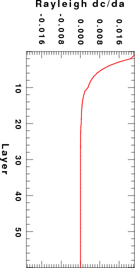
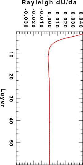
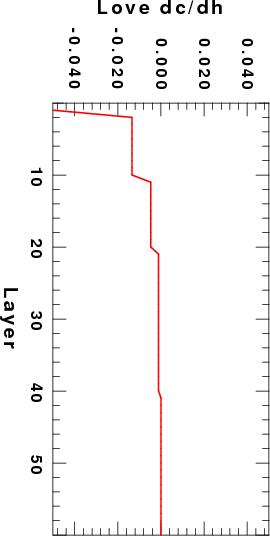
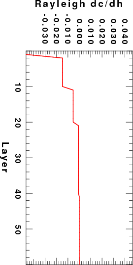
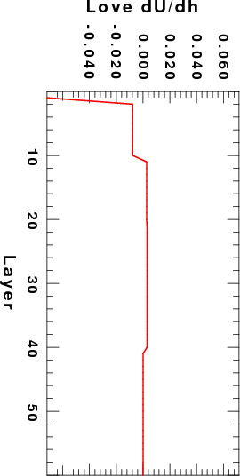
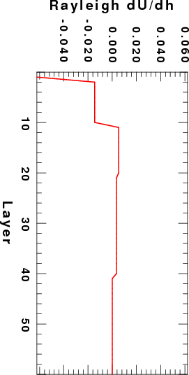
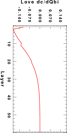
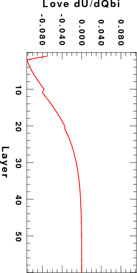
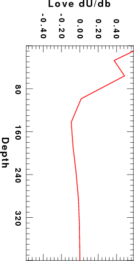
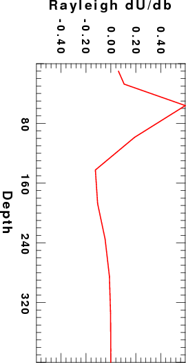
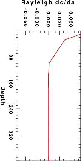
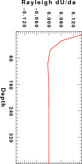
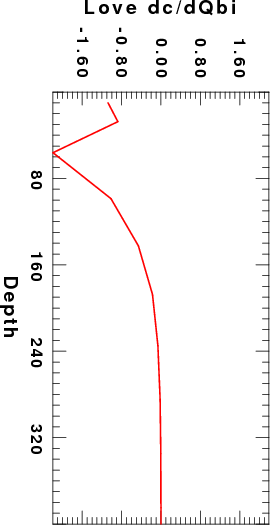
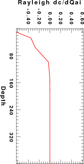
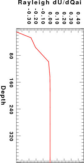
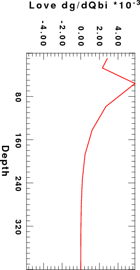
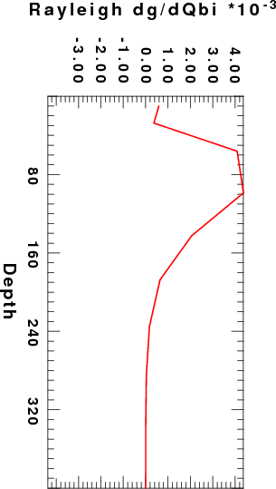
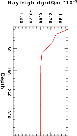
No program was written to make nice plots. Rather I used the script DOPLT in EXAMPLE_2 to make the following figures for the fundamental modes at a period of 10 seconds. Since the layers were 10 km thick, the Layer index is essentially the depth in km. Note that this is not the best plot since a staircase plot, similar to velocity models should actually be used.

Testing

To test the programs I modified the subroutine jsamat.f in PROGRAMS.330/VOLIV/src to create a file tmpjsamat.f. I also created a tMakefile to create a program tsurf96. The reason for the changes is that I wanted to determine the partial derivatives of the Rayleigh wave phase- and group velocity and anelastic attenuation coefficient with respect to changes in P- and S-wave inverse Q. The program surf96 assumes a specific fixed relationship between the inverse Q's ,a thus the effect of changing only one affects both partials.

To run the testing code, cd DIST/Source ; cp tMakefile tmpjsamat Your_Location/PROGRAMS.330/VOLIV/src
Then cd Your_Location/PROGRAMS.330/VOLIV/src, and then
make -f tsurf96

Now run the scripts in DIST/TEST

There are two scripts: DOPAR and DONUM

The idea is to create a set of models with perturbations in Vp, Vs, Layer Thickness, Qp and Qs. Then we use tsurf96 for each model to compute the dispersion parameters for the model, Finally the partial derivatives are determined numerically and compared with the output of srfker96. Computing partial derivatives is an art since one has to trade-off the numerical insensitivity to small changes with the non-linear effect if the change is too large. The initial part of DOPAR defines the perturbation in the medium velocities (km/s). inverse Q, and layer thickness (km). DOPAR then calls DONUM, and upon the completion of that program, numerically computes the partial derivatives.

DONUM works with three files: top.mod, 0.mod and bot.mod. If one applies the command

cat top.mod 0.mod bot.mod > model.0

The reference velocity model is created in the proper CPS format.

DONUM creates the files model.0, model.1 (Vp changed), model.2 (Vs changed), model.3 (Qp inverse changed), model.4 (Qs inverse-changed) and model.5 (layer thickness changed). Each model is run with tsurf96 to create the output files 0.OUT, ..., 5.OUT used by DOPAR. These files list the observed and predicted values. There are two new types of dispersion values, ga and gb, which give the effect of the Qp and Qs contributions to the anelastic attenuation coefficient (surf96 combines the effects by assuming a fixed ratio of Qp/Qs). The top part of DONUM creates the dispersion file, tdisp.d - this is where I change the period.

This run changes just the parameters in the second layer of the model. Byediting top.mod, 0.mod and bot.mod computations can be made for the other layers.

The output of DOPAR can be compared directly to the output of srfker96. In the listing below, I have added the DOPAR output (in RED) immediately after the corresponding line to the srfker96.txt file

Elastic  Love wave:     Period=    14.200 Mode =    0 C=     3.637 U=     3.405
LAYER    THICK     dc/db      dU/db      dc/dh      dU/dh
    1    20.000  7.724E-01  8.195E-01 -6.194E-03  3.115E-03
    2    20.000  3.027E-01  1.728E-01 -6.194E-03  3.115E-03
    3     0.000  2.583E-02 -4.096E-02  0.000E+00  0.000E+00
___________________________________________________________________________________________
Anelastic Love wave:     Period=    14.200 Mode =    0 C=     3.604 U=     3.383 GAMMA=  6.498E-04
LAYER    THICK     dc/db      dU/db      dc/dh      dU/dh     dc/dQbi    dU/dQbi    dg/dQbi
    1    20.000  7.659E-01  8.156E-01 -6.194E-03  3.115E-03 -2.283E+00 -1.520E+00  4.523E-02
    2    20.000  3.001E-01  1.705E-01 -6.194E-03  3.115E-03 -8.947E-01 -5.955E-01  1.772E-02
                 3.041e-01  1.859e-01 -5.853e-03  3.199e-03 -8.947e-01 -5.955e-01  1.772e-02
    3     0.000  2.561E-02 -4.145E-02  0.000E+00  0.000E+00 -1.025E-01 -6.824E-02  2.031E-03
___________________________________________________________________________________________
Elastic  Rayleigh wave: Period=    14.200 Mode =    0 C=     3.262 U=     3.080
LAYER    THICK     dc/da      dc/db      dU/da      dU/db      dC/dh      dU/dh
    1    20.000  8.013E-02  5.143E-01  4.639E-02  8.997E-01 -4.813E-03  1.197E-02
    2    20.000  3.168E-03  3.086E-01 -1.292E-02 -1.442E-01 -4.813E-03  1.197E-02
    3     0.000  1.064E-04  1.392E-02 -5.494E-04 -5.162E-02  0.000E+00  0.000E+00
___________________________________________________________________________________________
Anelastic Rayleigh wave: Period=    14.200 Mode =    0 C=     3.233 U=     3.061 GAMMA=  7.183E-04
LAYER    THICK     dc/da      dc/db      dU/da      dU/db      dc/dh      dU/dh     dc/dQai    dc/dQbi    dU/dQai    dU/dQbi    dg/dQai    dg/dQbi
    1    20.000  7.946E-02  5.099E-01  4.578E-02  8.991E-01 -4.813E-03  1.197E-02 -4.128E-01 -1.520E+00 -2.728E-01 -1.005E+00  1.016E-02  3.743E-02
    2    20.000  3.141E-03  3.060E-01 -1.303E-02 -1.482E-01 -4.813E-03  1.197E-02 -1.632E-02 -9.122E-01 -1.079E-02 -6.028E-01  4.018E-04  2.246E-02
                 3.028e-03  3.029e-01 -1.330e-02 -1.504e-01 -4.341e-03  1.171e-02 -1.633e-02 -9.122e-01 -1.080e-02 -6.028e-01  4.018e-04  2.246e-02
    3     0.000  1.055E-04  1.380E-02 -5.535E-04 -5.204E-02  0.000E+00  0.000E+00 -7.326E-04 -5.526E-02 -4.841E-04 -3.652E-02  1.804E-05  1.361E-03
___________________________________________________________________________________________

As of the creating of this document I have not checked this with a spherical model, but everything should work.
This effort took several weeks of deriving all of the equations, writing the code and testing.

Example 3 - Kernels as a function of depth

The kernels given in the Computer Programs in Seismology 3.30 (CPS330) by the programs slegn96/sregn96/sdpder96 differ from those given in papers by Saito anbd others in a significant way. Those papers give the kernel at a given depth. The CPS330 values are the kernels for a given layer, which are obtained from the depth kernels through integration:

Kernel(CPS330) = integral_over_layer_of thickness_H Kernel(depth) dz.

Thus the kernel values given here will be larger than those of Saito by a factor related to the layer thickness.

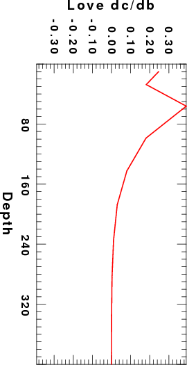
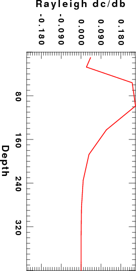
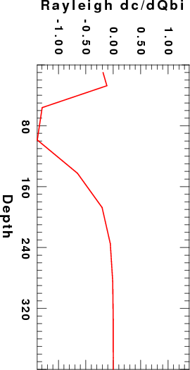
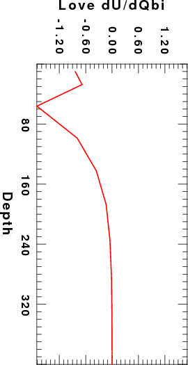
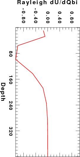
The following example computes the kernels using a modified AK135 velocity model, modified since the liquid core is ignored. The data set is in the subdirectory EXAMPLE_3. The other difference is that the plot of the kernels is as a function of the depth of the mid-point of the layer.

To make these plots, execute the following commands:

surf96 39
surf96 1
srfker96 > srfker96.txt
surf96 39
DOPLTz   
#(note that the script DOPLTz forces 
# the maximum depth to be 400 km)

If you look at the sobs.d file in EXAMPLE_3 you will see that the dispersion file is for a single period of 50 seconds. If you wish to see the kernels for other periods, just extract the Love and Rayleigh group velocities from the file out.dsp and place them in the tdisp used by surf96.