Computer Programs in Seismology

Waveform modeling

Introduction

The Utah earthquake of 2025/09/10 23:57:47 is interesting because the network depth was 69.4km and the SLU moment tensor depth was 64km. Such a deep event is rare in most of the continent interior. The moment tensor solution is detailed as https://www.eas.slu.edu/eqc/eqc_mt/MECH.NA/MECH.NA.2025/20250910235747/HTML.REG/index.html .

From the point of view of modeling an accelerometer was located within an epicentral distance of 15 km, and it may be interesting to model the waveforms at frequencies greater than the 0.05-0.15 Hz band used for the moment tensor inversion.

Observed data

the following shell scripts were used to prepare the observed data:

DOWS - Download all waveform data within 1 arc degree of the epicenter. Place the event location into the sac file headers and synchronize the time stamp so that 'O' (origin time offset) is 0.0
DODECON - Deconvolve the instrument response in the passband of 0.025 H to the 1/2 the Nyquist frequency. The results are placed in the sub-directory named GOOD
DOROT - Rotate the traces to Z R and T, and then put the predicted P and S times into the trace headers. The rotated ground velocities in units of m/s are in the sub-directory FINAL.

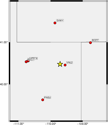
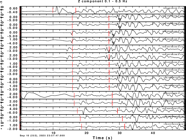
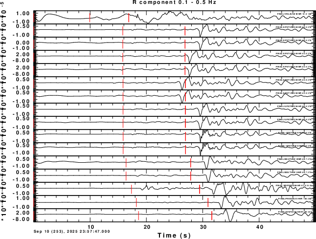
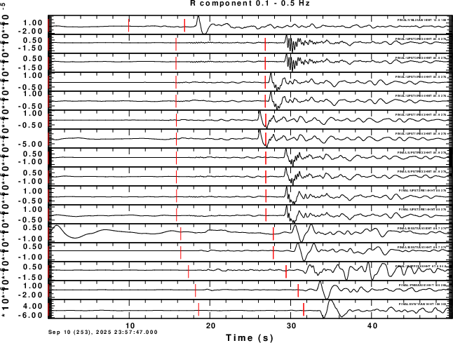
The DOROT scripts uses gsac to make trace plots and to create a shell script (map5.sh) that uses GMT to make a map showing the epicenter and the stations. The trace plots are in order in increasing epicentral distance. These figures are shown here.

Examining the traces, note that UPST3 and UPST4 arrives seem to arrive early early This is easily seen by focusing on the first red tic, which indicates the predicted P time. the P arrival of the other stations occurs about 1-2 seconds after this red marker. The lack of agreement just indicates that the velocity WUS velocity model may not be appropriate for this region. Perhaps there is a clock problem at UPST3 and UPST4.

For the purpose of modeling, only the accelerometer data at VNL2 (distance of 13.5 km) and BSUT (distance of 89.7km). The details are

  Waveform   Epicentral Distance 9km)   Azimuth
VNL2UU01ENR          13.48988             99.97
VNL2UU01ENT          13.48988             99.97
VNL2UU01ENZ          13.48988             99.97
BSUTUU01HHR          89.73962            274.35
BSUTUU01HHT          89.73962            274.35
BSUTUU01HHZ          89.73962            274.35

Green's functions

In order to compare the observed waveforms to model based predictions, it is necessary to compute the Green's functions. The organization for the Green's functions is given MakeGreen.tgz. To unpack and compute the Green's functions, do the following:

gunzip -c MakeGreen.tgz | tar xf - 
cd GREEN/nWUSHF.REG
DOIT.WKdeep

The DOIT.WKdeep will compute Green's functions for the WUS.mod at source depths of 5, 10, ..., 75 and 80 km. After the computations are completed, the nWUSHF.REG directory will appear as this when using the 'ls -F' listing command:

0050/	0250/	0450/	0650/	DOIT.WKdeep*
0100/	0300/	0500/	0700/	MKW*
0150/	0350/	0550/	0750/	Model/
0200/	0400/	0600/	0800/	WUS.mod

The naming convention is such that the 0600 directory contains the Green's functions for a 60.0 km source depth. Th contents of the 0600 directory will be

001400600.RDD 001400600.TSS 009000600.RDD 009000600.TSS dfile
001400600.RDS 001400600.ZDD 009000600.RDS 009000600.ZDD hspec96.dat
001400600.REX 001400600.ZDS 009000600.REX 009000600.ZDS hspec96.grn
001400600.RSS 001400600.ZEX 009000600.RSS 009000600.ZEX W.CTL
001400600.TDS 001400600.ZSS 009000600.TDS 009000600.ZSS

The naming convention created by the use of the f96tosac -G command is DDDDdHHHh.GRN, which represents an epicentral distance of DDDD.d km and a source depth of HHH.h km.

The DOIT.WKdeep script created 1024 sample long time series with a sampling interval of 0.05s. The source time function has a duration of 0.2s. For the model parameters used, the Green's functions represent ground velocity in cm/s for a unit step-like source time function with a moment of 1.0e+20 dyne-cm.

Modeling

Assuming that your top level directory now contains DODECON, DOROT, DOWS, MakeGreen.tgz, GOOD/ FINAL/ GREEN/ and the original files from the data center, the synthetic seismogram scripts will assume that the Green's functions are in GREEN/nWUSHF.REG. h

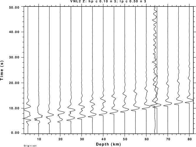
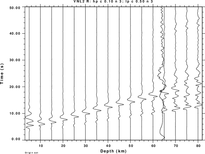
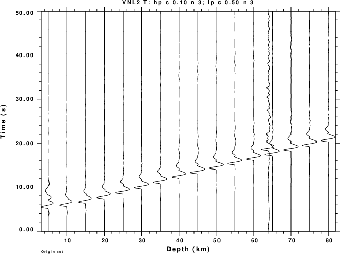
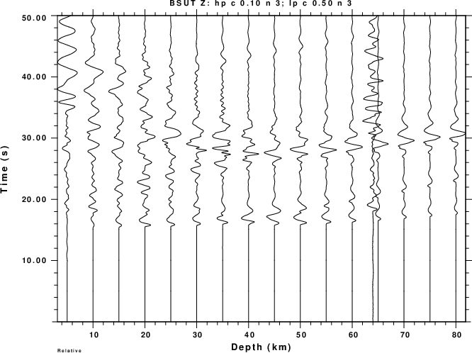
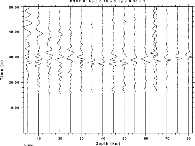
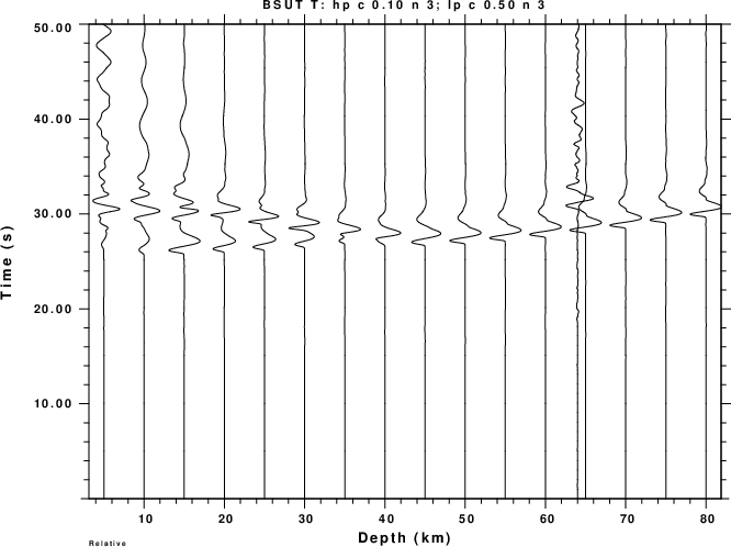
The annotated scripts DODEPTHVNL2 and DODEPTHBSUT compute mechanism predicted ground velocities from the Green's functions for each station. These are then compared to the observed waveforms. The plots are filtered ground velocity. However true amplitude are not displayed. Note the display would be better if I had picked the P arrival on the observed waveforms and then aligned the traces with P.

VLN2 - Z VLN2 - R VLN2 - T

BSUT - Z BSUT - R BSUT - T

Discussion

The R component at VLN2 is noisy. If this trace is filtered "hp c 0.1 n 3 ; lp c 1.0 n 3" there are nice P pulses on the Z and . There is a slight delay in the P on the R compared to the Z. This could be due to some conversion of P -> S -> R along the path. There is little P on the T component. So the azimuth to the station an station component orientation can be accepted. The peak P amplitudes are 1.2e-5 m/s on R and 1.1e-4 on Z. Assuming surface velocities, the R/Z amplitude ration could be used to define the ray parameter of the P-wave which might be useful is pinning down the depth, by search for the depth that corresponds to a ray appearing at an epicentral distance of 14 km.

Another test with synthetics would be to find the depths where the S arrival on the R component is a single pulse.

The scripts can be modified to test other velocity models. Note that all synthetic depths are with respect to the surface of the model, which is also true for the moment tensor depth since it is based on synthetics. Network depths are relative to mean sea level.

Finally no attempt was made to address the source time function. which may be shorter than the 0.2s used for the Green's functions.