Computer Programs in Seismology Tutorial

Introduction

The purpose of this tutorial is to model strain and displacement at DAS elements of an actual array. thus it differs from the tutorial CPSstrain in that example can be modified to model actual data sets.

The file ../CPSSTRAIN/strain.pdf describes the theory of the CPS codes used to model the displacement, strain and stress fields.

Coordinate systems

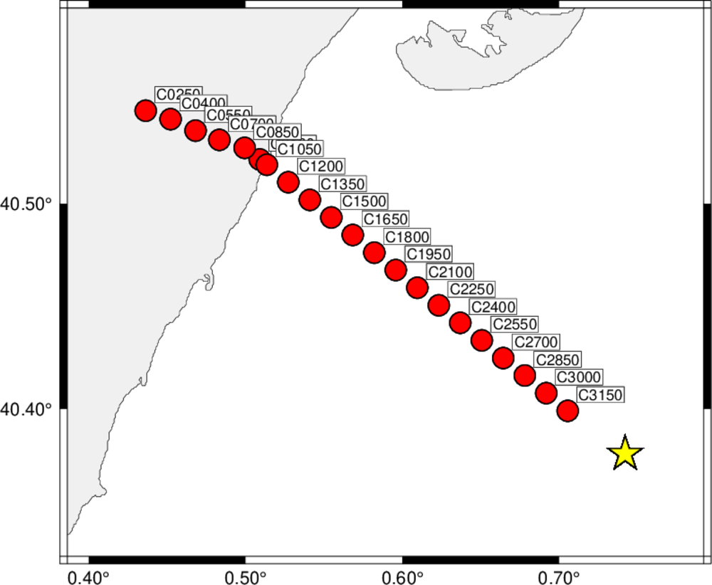
The following figures illustrate the geometry of the problem and the angles involved. The epicenter generates the seismic wavefield which then propagates to the DAS element. At distances short enough that one can ignore the curvature of the earth, the back azimuth from the DAS element to the epicenter is just 180^o plus azimuth from the source. When this is not true, then this simple relation does not hold.

The x_r, x_φ, x_z and x₁, x₂, x₃ are right-hand coordinate systems with the x_z and x₃ axes positive downward.

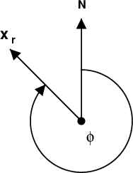
Figure 1 illustrates the coordinate that governs the radiation of the source. The great circle path from the source to the receiver leaves the source at an azimuth of φ.

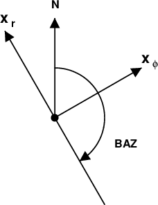
Figure 2 displays the coordinate system at the receiver. x_r is the direction of the incident ray from the source. The azimuth from the source, φ and back azimuth, BAZ, are computed given the geographic coordinates of the source (ELAT,ELON) and receiver (STLA, STLO).

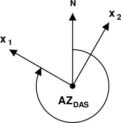
Figure 3 describes the orientation of the DAS element. In the presentation here, the DAS element is aligned with the x₁ axis, which trends in a direction defined by AZ_DAS.

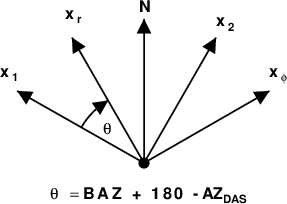
Figure 4 shows the relationship between the incident wavefield and the DAS coordinate system. The angle θ = BAZ + 180 - AZ_DAS is used to transform the displacements, stresses and strains in the (r,φ,z) coordinate system tot he desired (1,2,3) coordinate system.

φ - azimuth with respect to North from the source to the receiver. The angle φ affects the radiation pattern from the source.
BAZ - back-azimuth with respect to North from the receiver back to the source. This angle is usually used to rotate observed horizontal motions to radial and transverse with respect to the incident ray. The radial direction away from the source is at an azimuth of π + BAZ .
AZDAS - direction of a local x1 axis at the receiver. We will assume that this is the local direction of the DAS line.
θ - angle from the positive x1 axis to the radial direction from the source.

All angles are measured in a clockwise direction

In order to model the observed U_x and e_xx at the DAS element, the following steps are performed:

• Compute the U_r, U_φ,U_z, e_rr, e_rφ, ..., e_zz at the DAS element.

• Rotate these into the coordinate system aligned with the DAS line to form the u₁ and e₁₁.

Detailed example

Download the DOSTRAIN.tgz and unpack it using the command

gunzip -c DASSTRAIN.tgz | tar xf - 

The will create the directory DASSTRAIN with shell scripts DOITWK and DOITSW. The first computes complete synthetics using wavenumber integration, while the second uses surface-wave modal superposition.

Wavenumber integration

cd DASSTRAIN
DOITWK

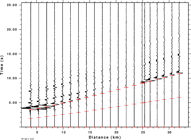
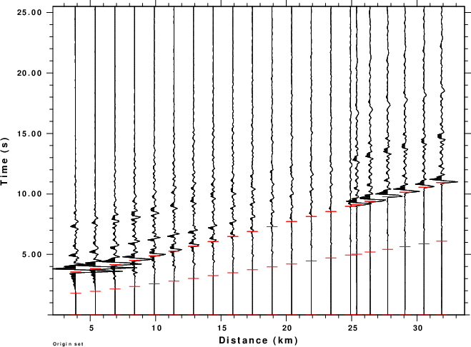
The script DOITWK is based on a real data set. The script consists of the following sections:

• Define the source hypocentral coordinates and mechanism
• Define the velocity model
• Starting with a tabulation of geographic coordinates of points on the DAS line, create a table of triplets of locations where the three entries define a linear section of the DAS line. The first and third sets define the horizontal orientation of the DAS line while the second set is used to define the distance from the source, the azimuth from the source to the element and the back-azimuth from the element to the source.
• For each DAS element, compute the ground velocity and strains at the element in the x_r, x_φ and x_z coordinate system and then rotate it to the DAS local coordinate system for each element. the result will be the desired E₁₁ strain and u₁.
displacement, or equivalently the E_xx and u_x which will be the output of hpulse96strain or spulse96strain.
• Finally make a map using GMT5+ showing the epicenter and DAS elements.

Modal superposition

cd DASSTRAIN
DOITSW

This script invokes the surface wave codes. Since the surface wave synthetic will include only those arrivals with phase velocities less than or equal to the halfspace S-wave velocity and since the example has the source in the medium where V_P is 6 km/s, the model used for the wavenumber integration will not be able to model the wavefield due to the direct P wave. To address this a layer is placed at depth with V_P=14 km/s and VS=7 km/s. The resulting synthetics are known as locked mode synthetics.

The next two figures overlay the wavenumebr integration and locked mode synthetics using different colors for each.. the comparison is excellent.

Discussion

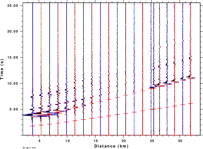
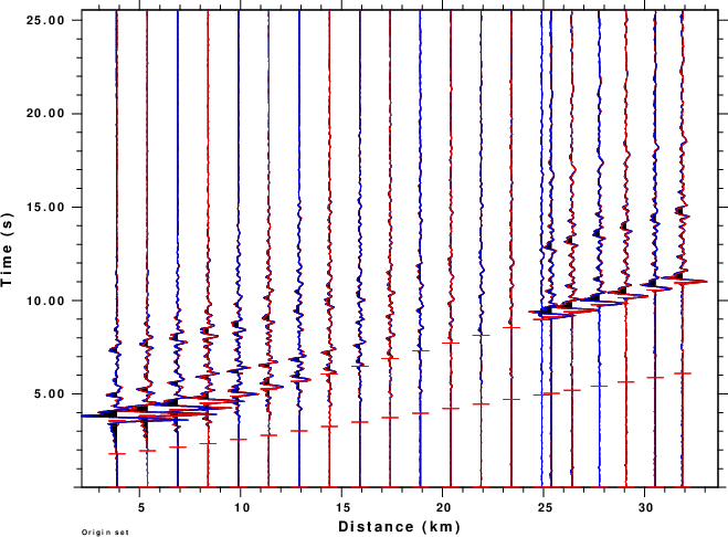
One interesting aspect of this study is that the initial P-wave amplitudes are very small for this source mechanism. Another interesting feature is that the E₁₁ is very similar in appearance to the u₁ ground velocity.

Support scripts

The scripts EPSTOPNG and DOPLTPNG are sued to convert EPS and the CPS PLT files to PNG bit graphics using the ImageMagick package convert. These were used to create the graphics of this tutorial.