Computer Programs in Seismology

Strain Synthetics - Tests

1. Introduction

This tutorial introduces the program hwhole96strain which is built upon hwhole96. Recall that hwhole96 provides the Fourier transform of the isotropic wholespace Green's functions for use with hpulse96. Since hwhole96 is based on an analytic solution, its output can be used to evaluate the wavenumber integration component of hspec96. These programs are executed as

hprep96 -M model -d dfile -HS 10 -HR 0 -ALL hspec96 hpulse96 -V -p -l 1 | f96tosac -G

hprep96 -M model -d dfile -HS 10 -HR 0 -ALL hwhole96 hpulse96 -V -p -l 1 | f96tosac -G

The hwhole96strain is the isotropic wholespace solution that can be used to evaluate hspec96strain. The use of each is illustrated by the comparison

hprep96 -M model -d dfile -HS 10 -HR 0 -ALL hspec96strain hpulse96strain -V -p -l 1 | f96tosac -G

hprep96 -M model -d dfile -HS 10 -HR 0 -ALL hwhole96strain hpulse96strain -V -p -l 1 | f96tosac -G

The tutorial Stress-strain synthetics describes the creation pf synthetics using the sequence: hprep96, hspec96strain and hpulse96strain.

Testing

This purpose of this tutorial is to use hwhole96 and hwhole96strain to illustrate problems with the current versions of hspec96 and hspec96strain. In addition hspec96strain is executed for a halfspace and for a layered halfspace to illustrate numerical problems. The testing focuses on a set of epicentral distance for a fixed source depth and a set of source depths for fixed epicentral distance. As will be seen, the current code has problems for some Green's functions at the vertical distance between the source and receiver is small.

An overview of the wavenumber integration and considerations in its implementation are given in the document Theory.pdf.

Discussion

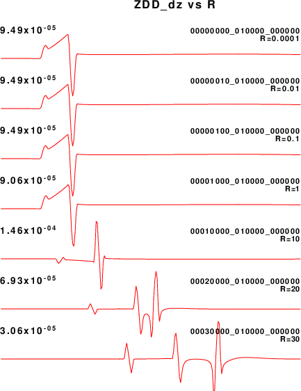
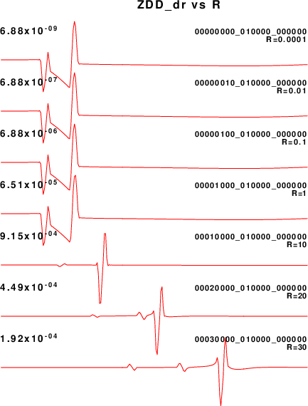
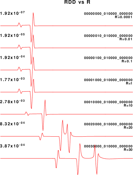
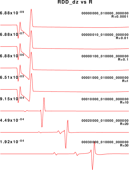
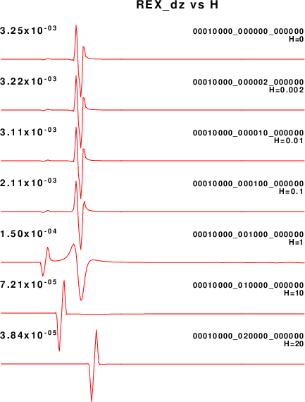
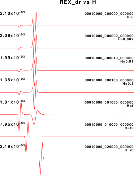
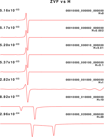
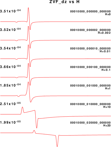
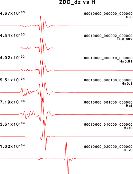
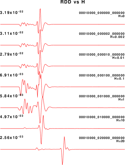
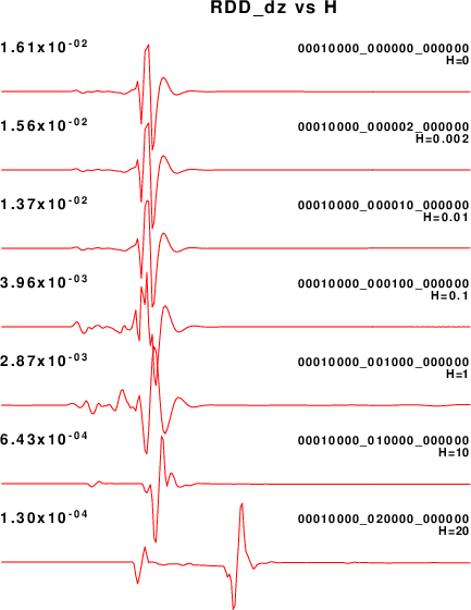
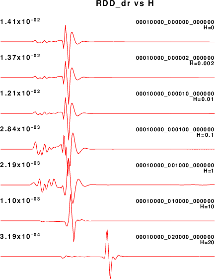
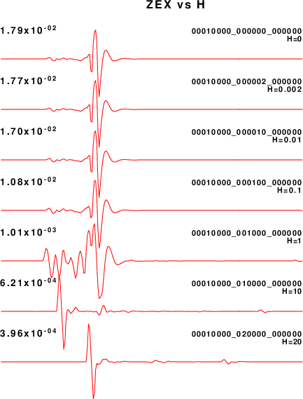
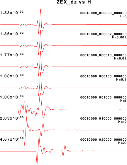
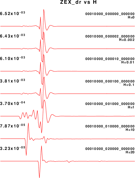
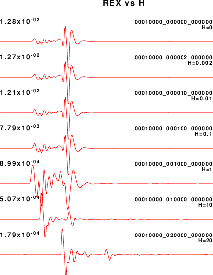
In this test run everything looks good, although there is no analytic solution for comparison. Because of the absence of the low frequency imperfections, it is easier to see how the amplitude of some of the Green's function derivatives tend to zero as the vertical distance becomes smaller.

Green's functions

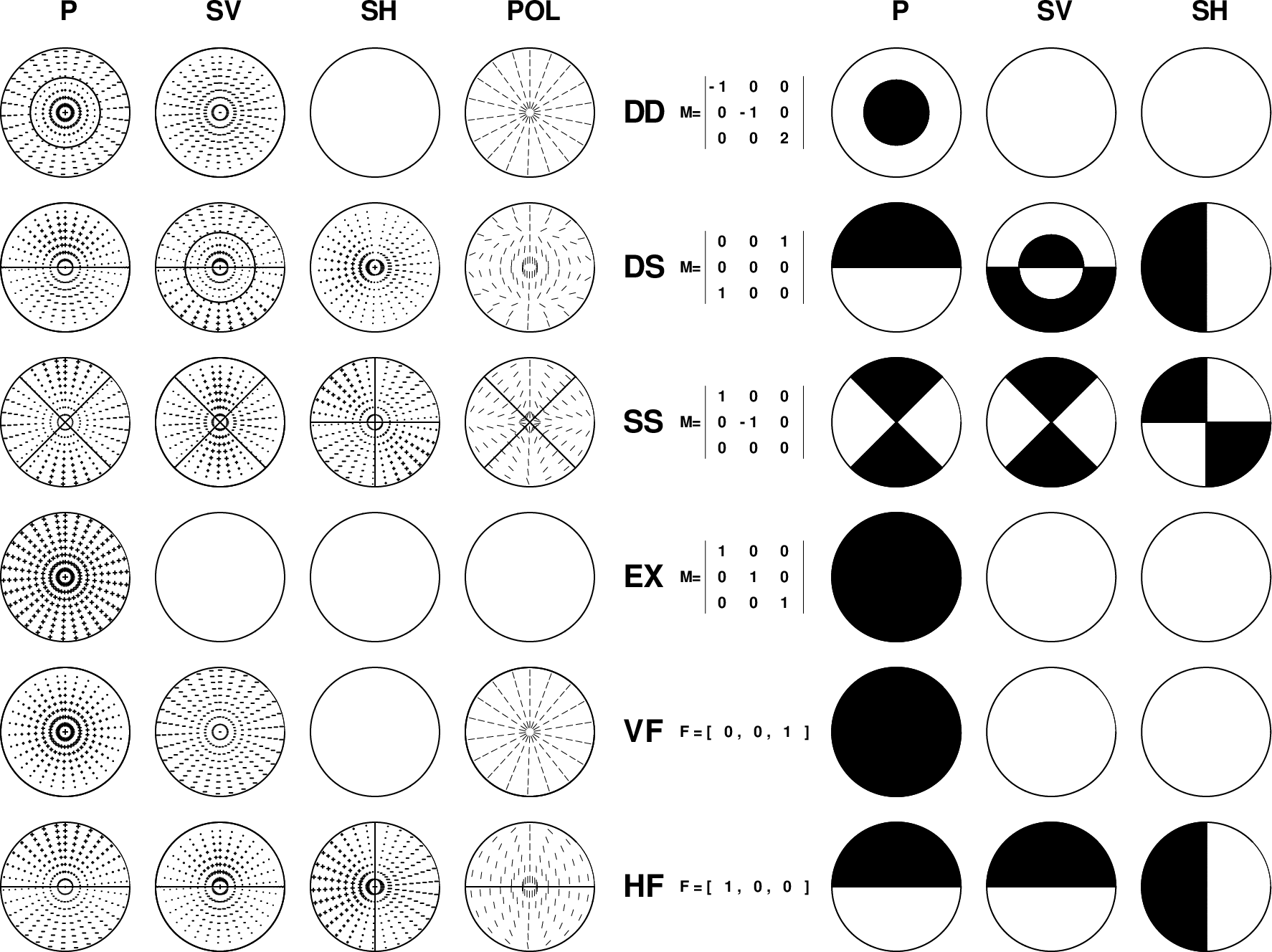
To assist in the the evaluation, the next figure displays the far-field body-wave radiation patterns. The center columns indicate the Green's function type, e.g., SS which will give the ZSS, RSS and TSS Green's function, and the corresponding moment tensor or force configuration. The other columns indicate the wave type, e.g., P, SV or SH, and S-wave polarization. The size of the +/- symbols on the left indicate the relative amplitudes, while the figures on the right indicate positive (black) and negative (white) polarities. Finally the blank figures on the left indicate that a wavetype is not generated, e.g., the EX source does not generate SV or SH, the DD source does not generate SH, and the VF, vertical force, source does not generate SH.

2. Stress test

The wavenumber integration code within hspec96, rspec96, tspec96 and hspec96strain often has numerical problems when the path of the direct arrival from the source to the receiver is nearly horizontal because the direct arrival is often has the largest amplitude and the small vertical offset means that the f(k,ω) does not decay rapidly as k → ∞. When the vertical offset is not zero, the decay occurs at high frequencies. The underlying difficulty is that wavenumber integration requires the evaluation of the integrals of the form ∫₀^∞ f ( k, ω ) J_n (k r ) dk, but this is approximated as ∫₀^Kmax f ( k, ω ) J_n (k r ) dk assuming that the contribution from [Kmax, ∞] is negligible. This truncation problem is worse at lower frequencies.

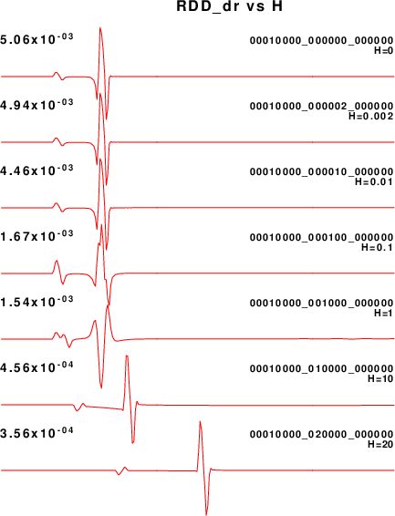
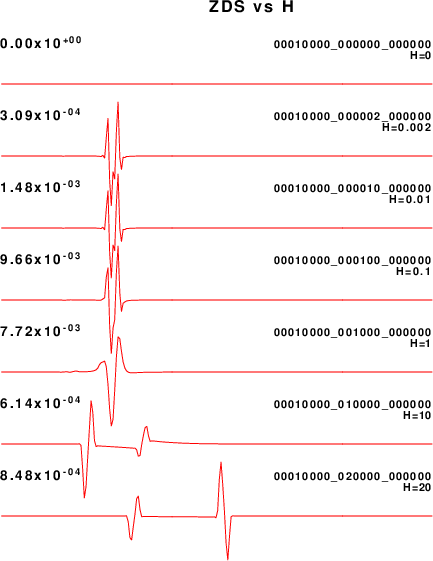
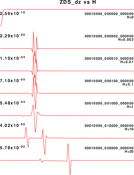
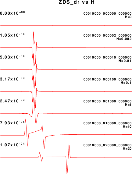
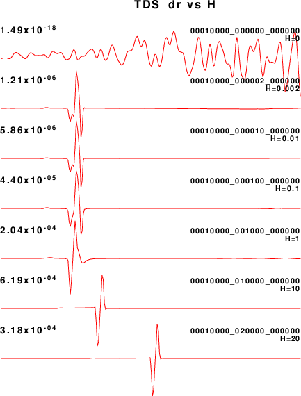
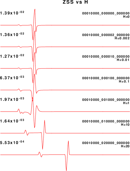
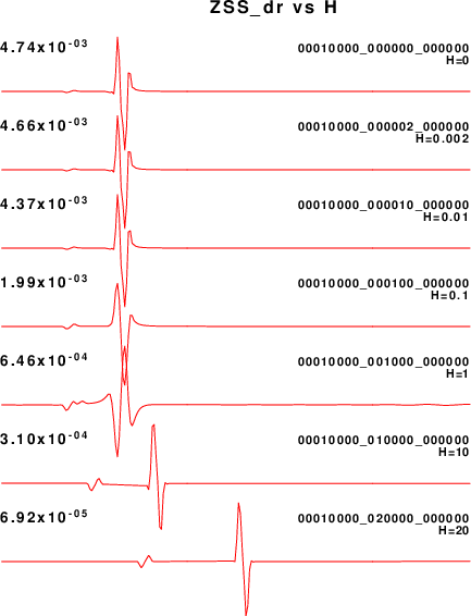
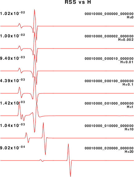
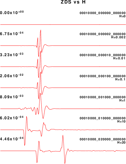
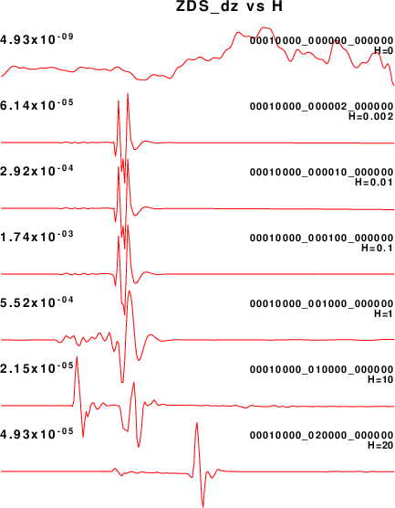
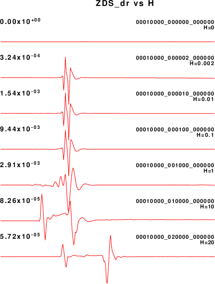
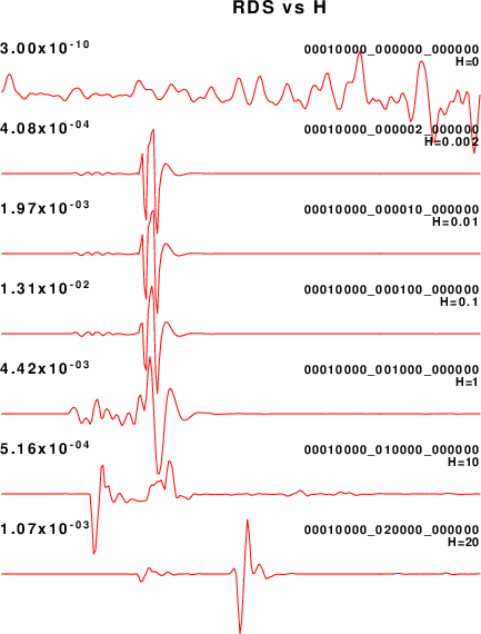
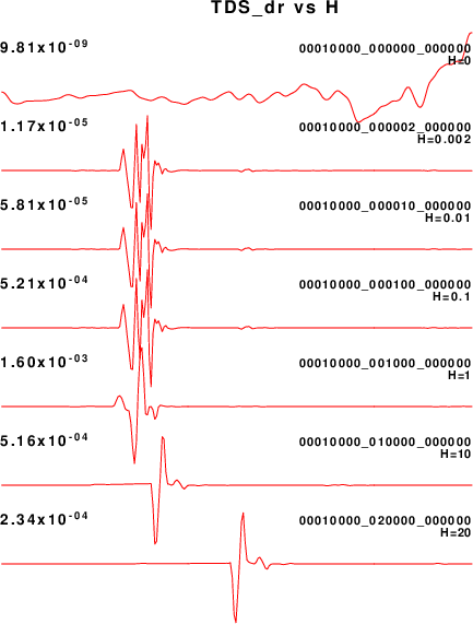
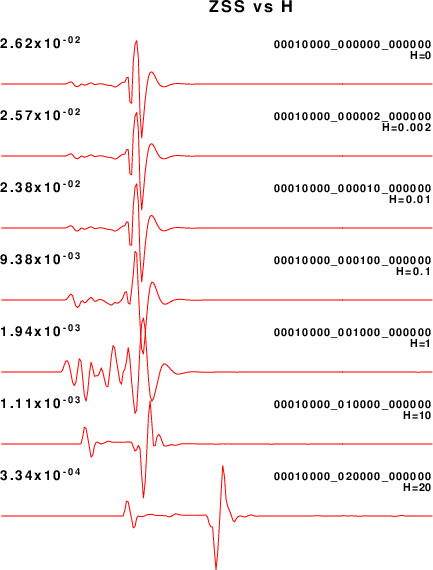
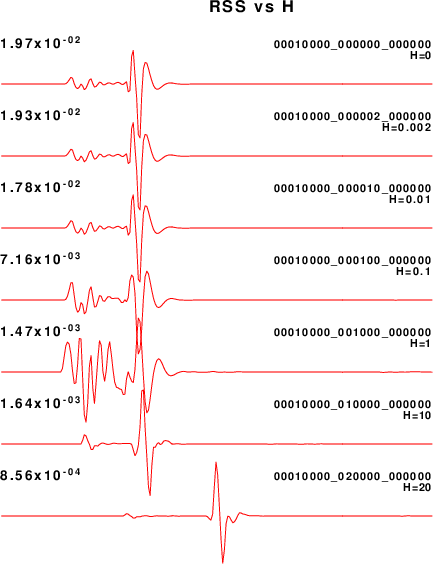
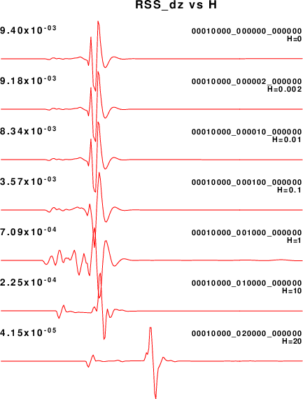
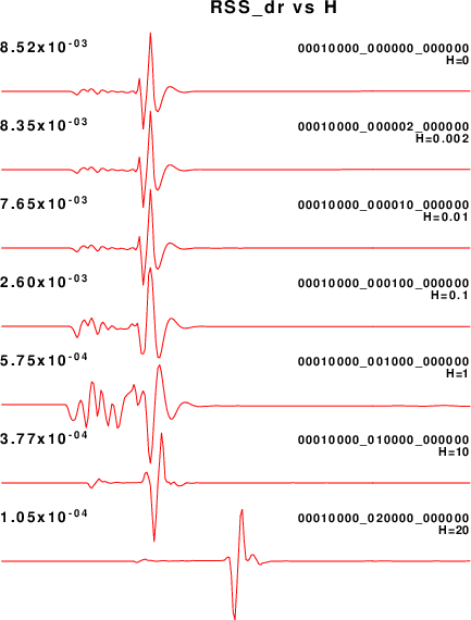
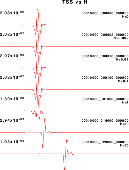
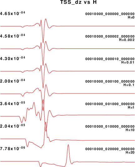
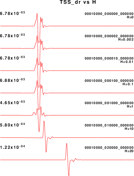
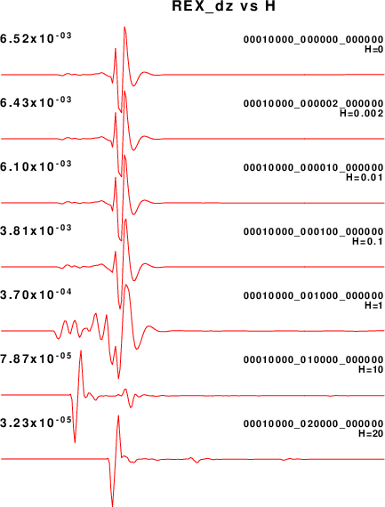
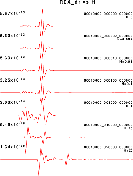
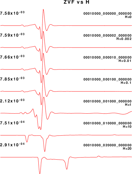
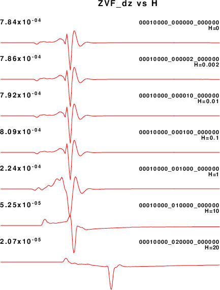
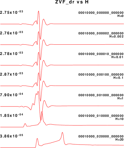
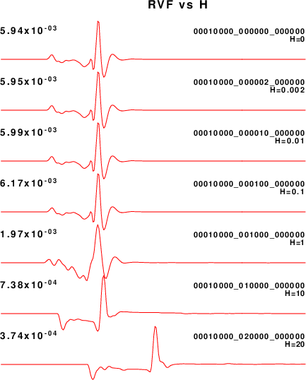
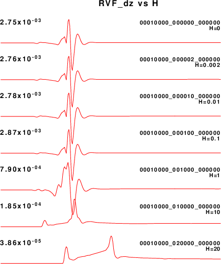
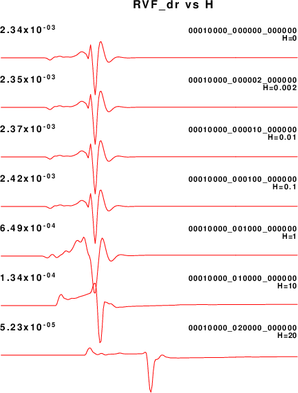
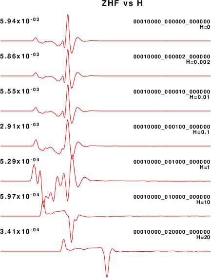
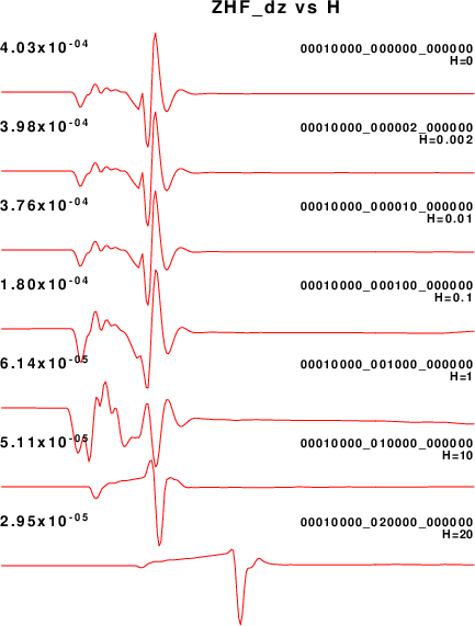
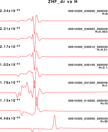
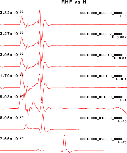
To test the current coding and to highlight problems, the Green's functions and partial derivatives with respect to the vertical and radial positions of the receiver are compared first with a fixed source depth of 10.0km and different epicentral distances and then for a fixed radial distance of 10.0 and different vertical distances between the source and the receiver. The use of hpulse96strain with the -TEST1 flag gives the Green's functions and the partial derivatives with respect to the receiver (r,z) coordinates. If these "look" good, then the strains, stresses and rotations computed will be OK. It is assumed that the computation of strain using the Green's functions and their derivatives with respect to 'r' and 'z' is correct (Stress-strain synthetics).

Wholespace Test

The wholespace velocity model, named W.mod is created with this shell script:


cat > W.mod << EOF
MODEL.01
Simple wholespace model
ISOTROPIC
KGS
FLAT EARTH
1-D
CONSTANT VELOCITY
LINE08
LINE09
LINE10
LINE11
H(KM) VP(KM/S) VS(KM/S) RHO(GM/CC) QP QS ETAP ETAS FREFP FREFS
40.0  6.00       3.5     2.7        0  0  0    0     1     1
EOF

The processing scripts used are called with the source depth and epicentral distance as command line arguments.

#!/bin/sh H=$1 R=$2 cat > dfile << EOF ${R} 0.05 256 0 0 EOF hprep96 -M W.mod -d dfile -HS ${H} -HR 0 -TH -BH hwhole96strain hpulse96strain -TEST1 -V -p -l 2 -FMT 2

#!/bin/sh H=$1 R=$2 cat > dfile << EOF ${R} 0.05 256 0 0 EOF hprep96 -M W.mod -d dfile -HS ${H} -HR 0 -TH -BH hspec96strain hpulse96strain -TEST1 -V -p -l 2 -FMT 2

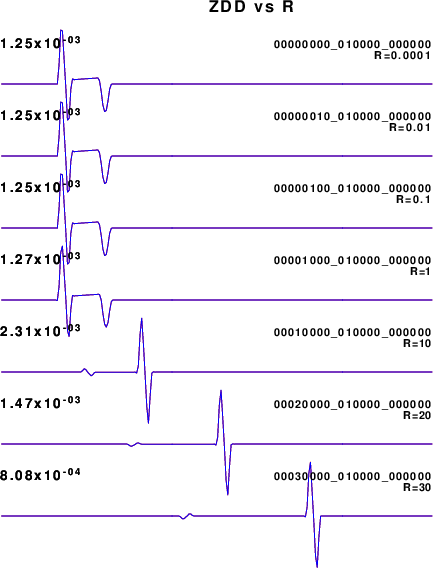
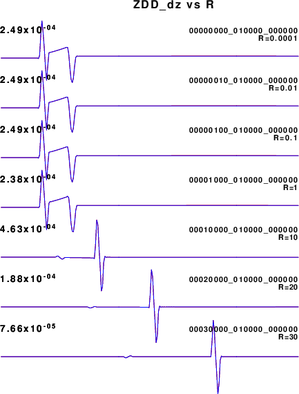
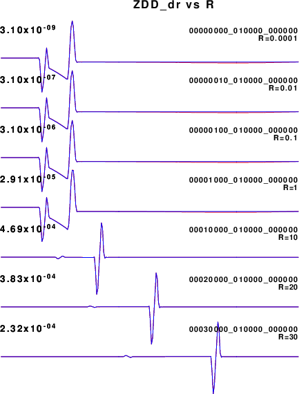
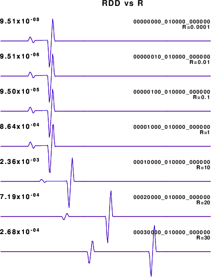
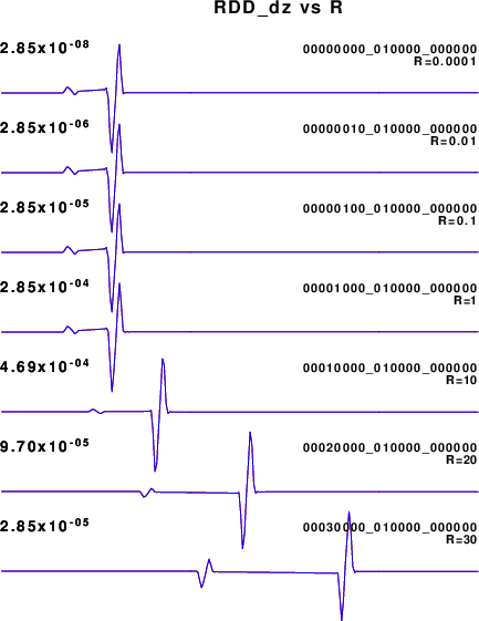
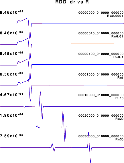
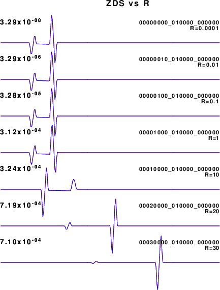
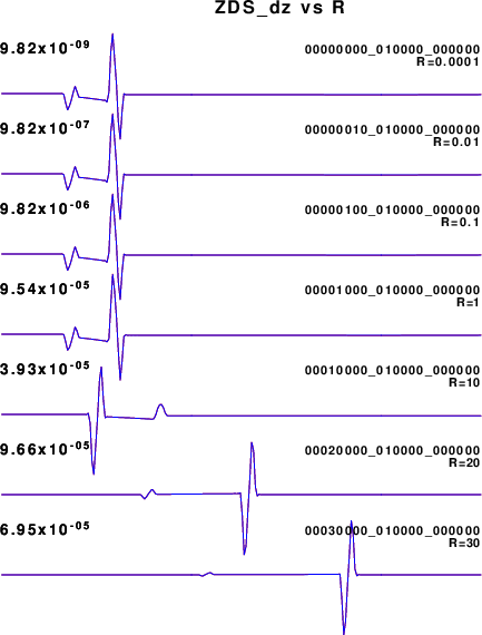
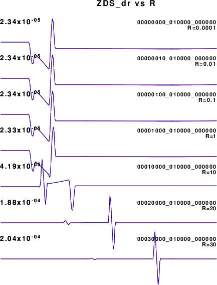
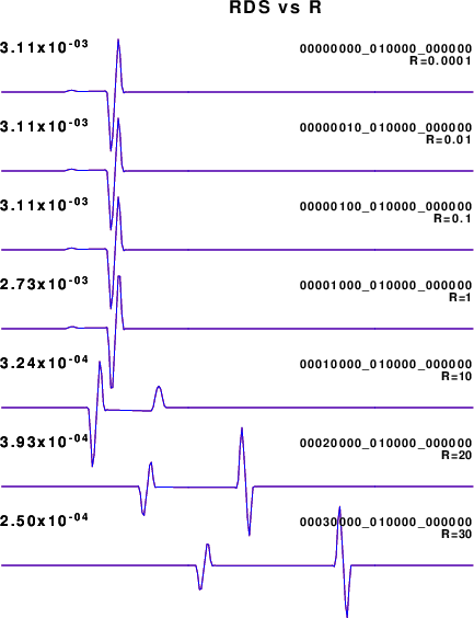
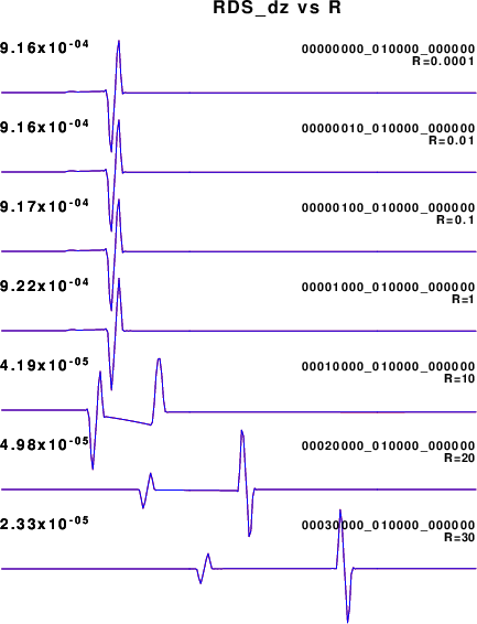
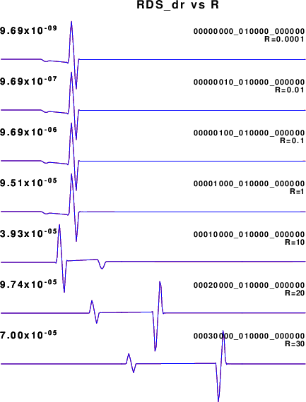
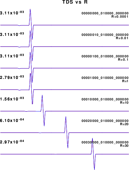
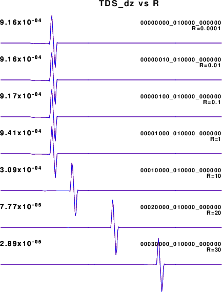
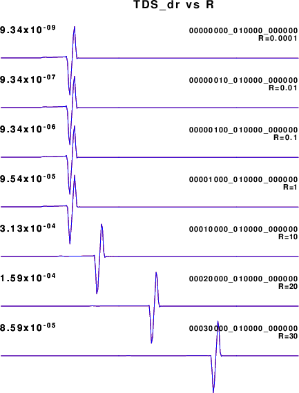
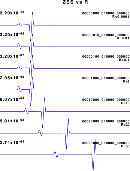
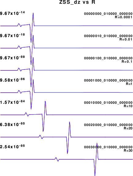
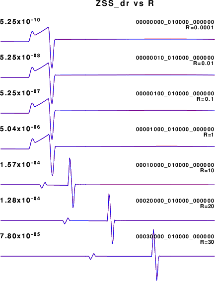
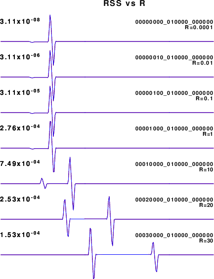
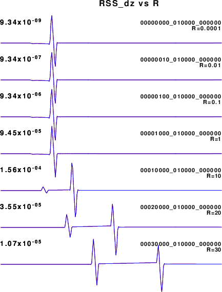
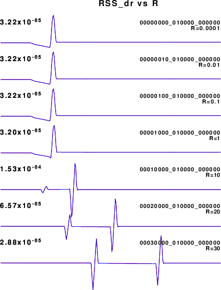
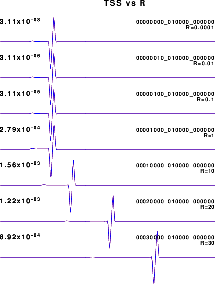
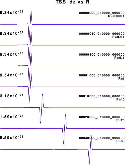
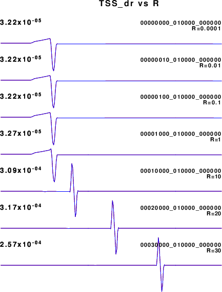
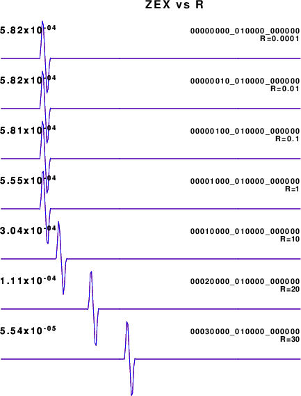
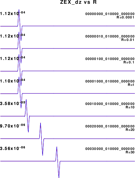
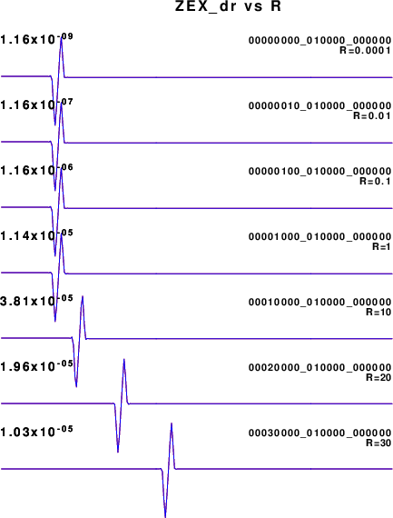
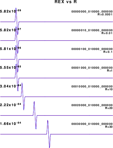
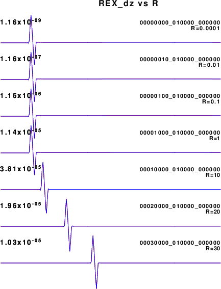
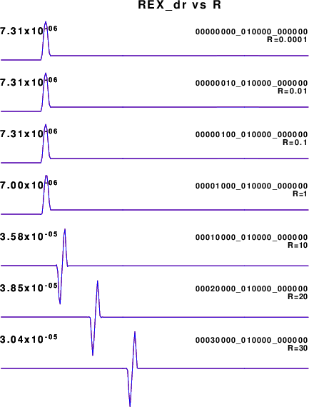
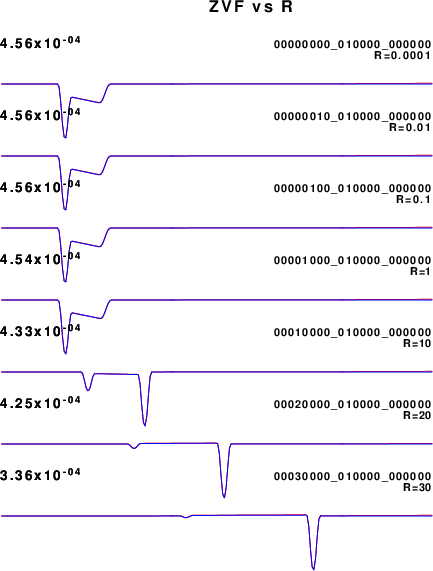
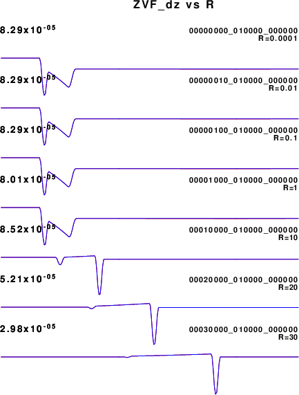
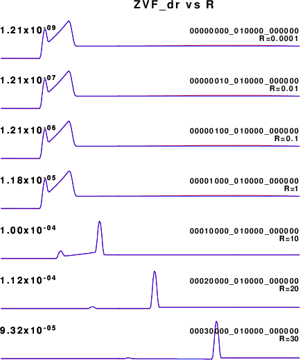
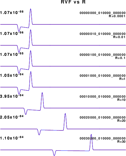
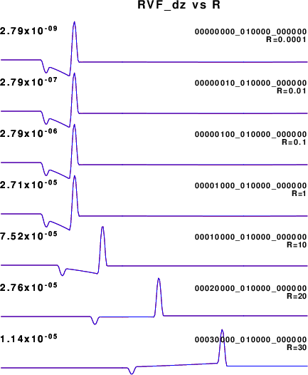
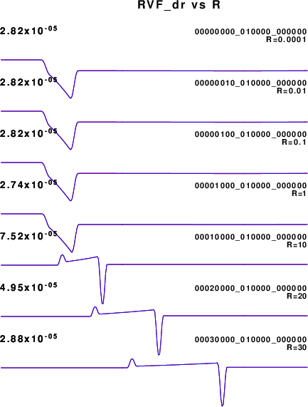
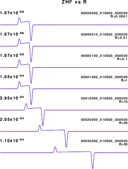
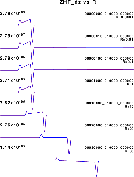
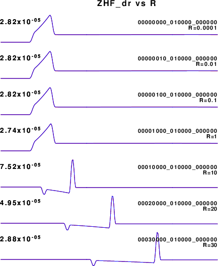
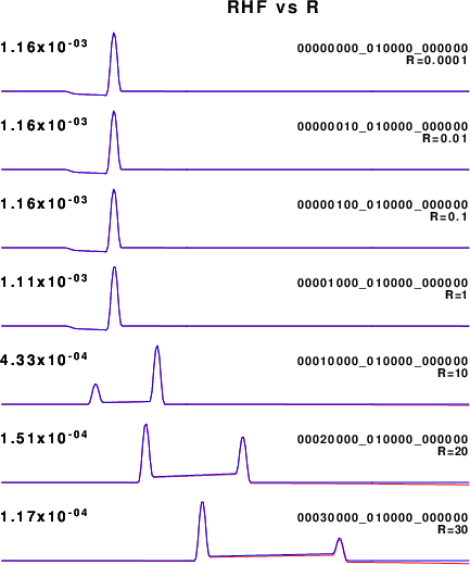
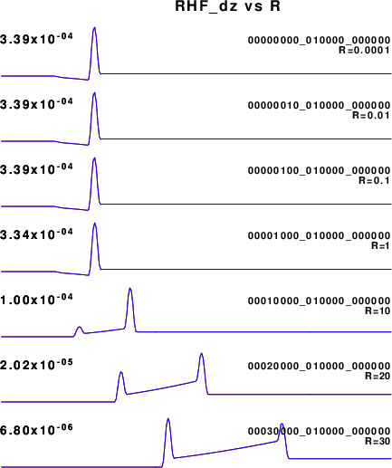
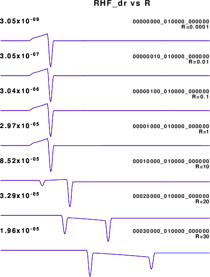
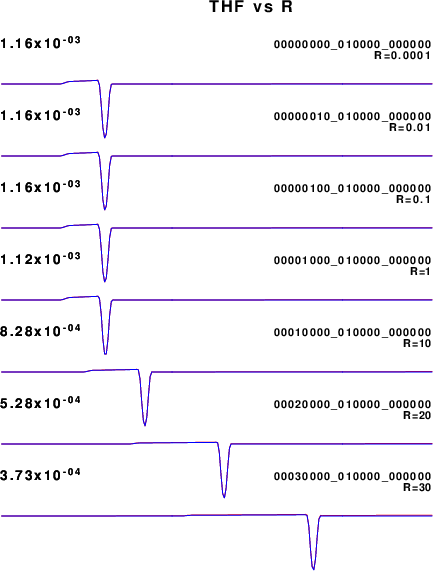
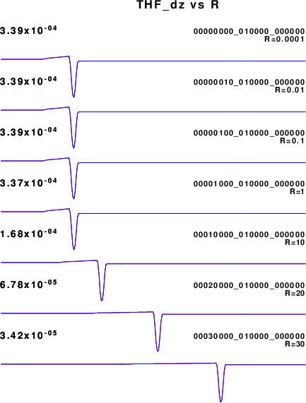
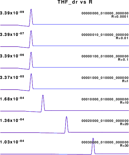
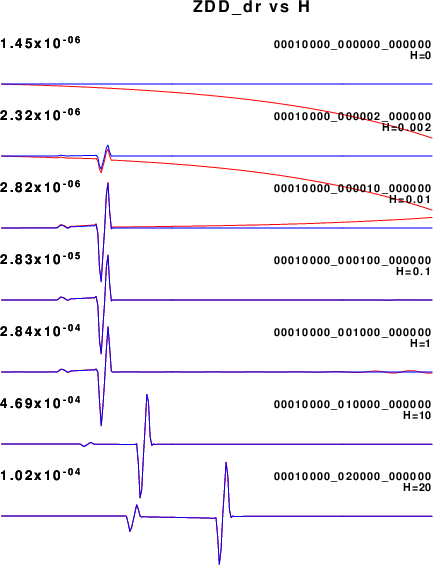
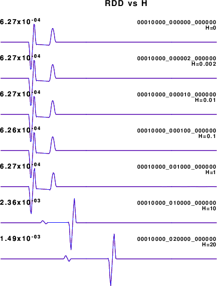
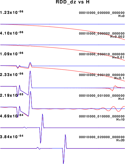
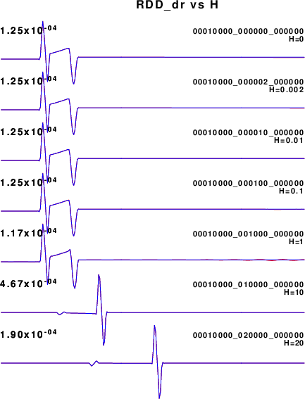
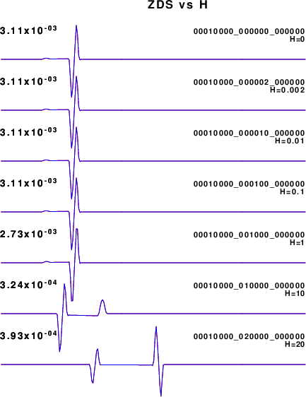
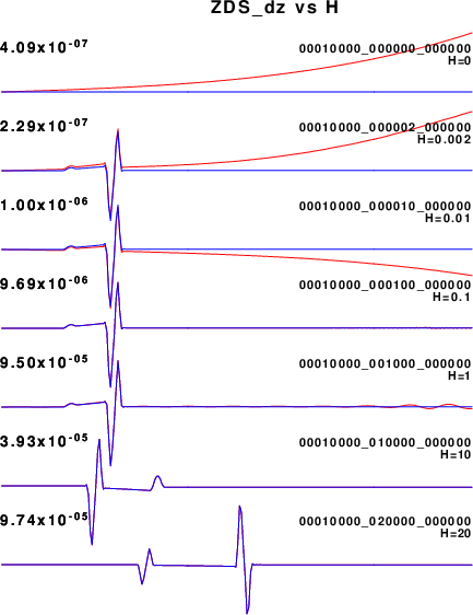
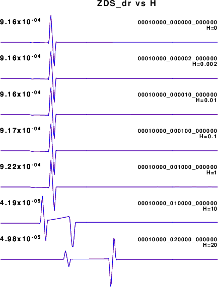
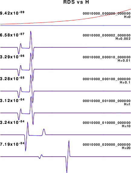
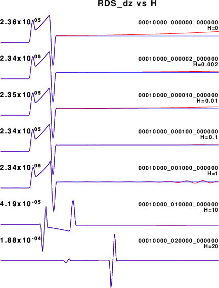
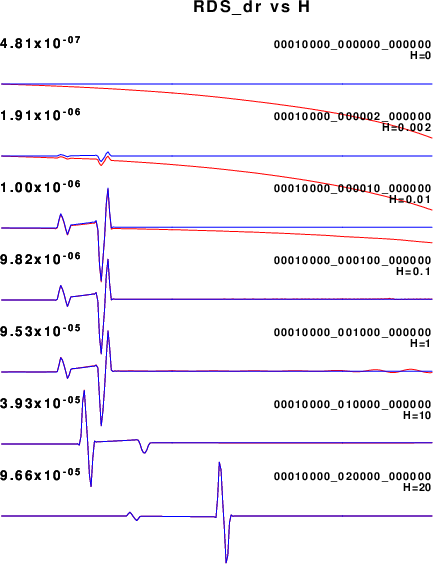
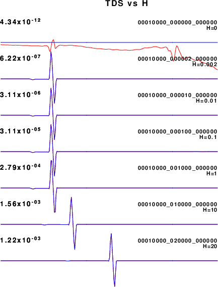
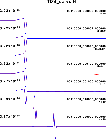
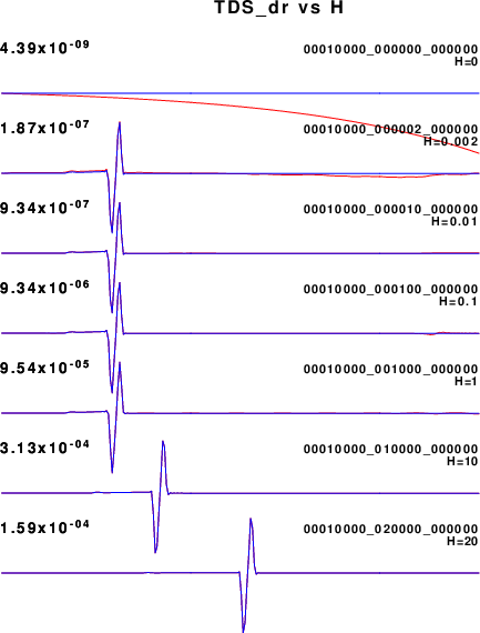
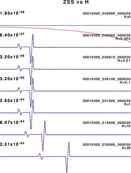
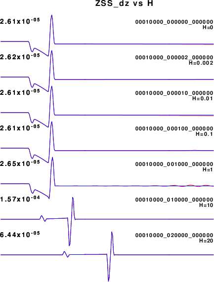
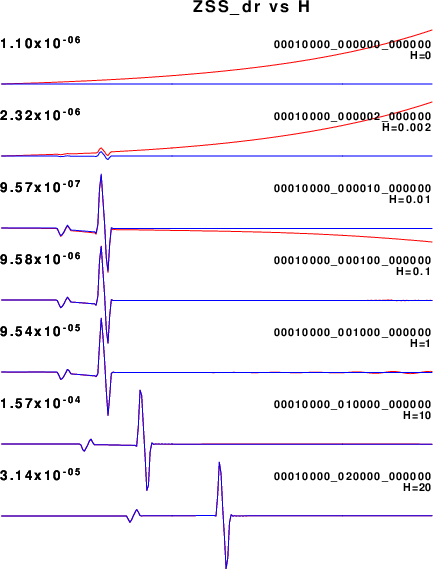
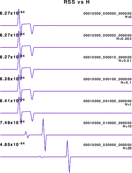
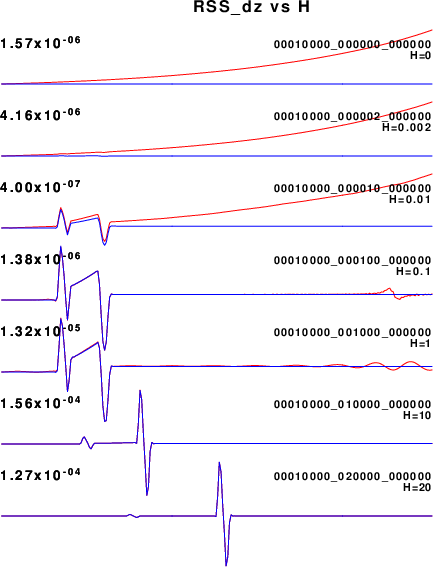
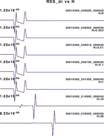
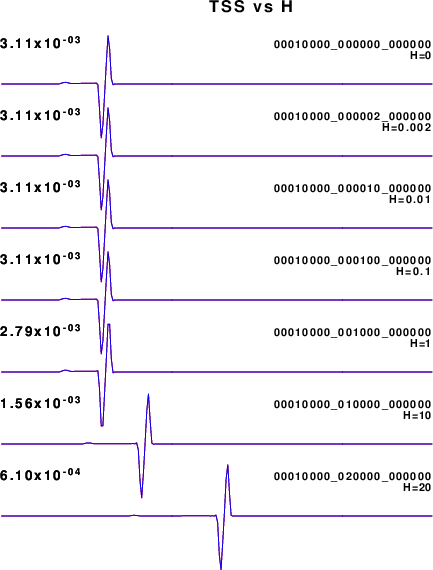
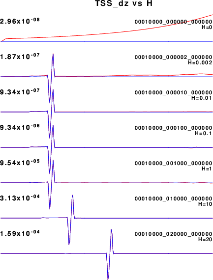
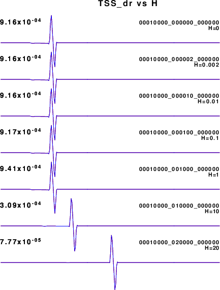
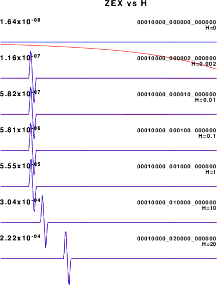
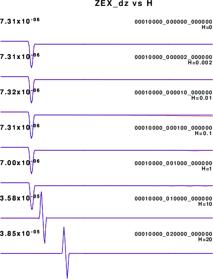
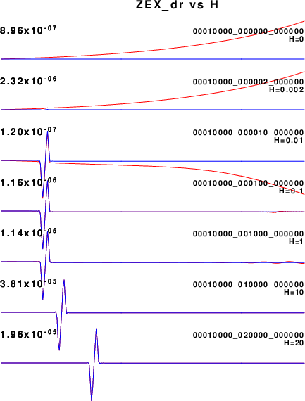
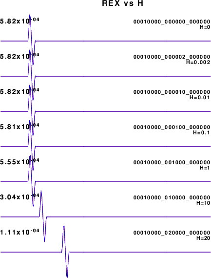
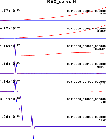
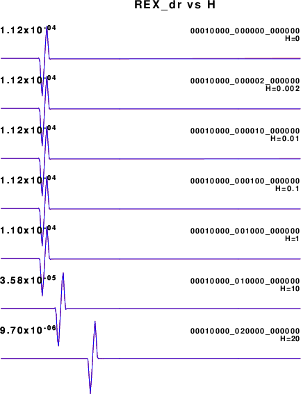
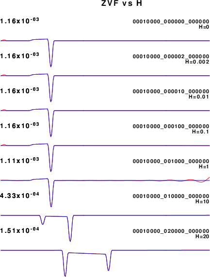
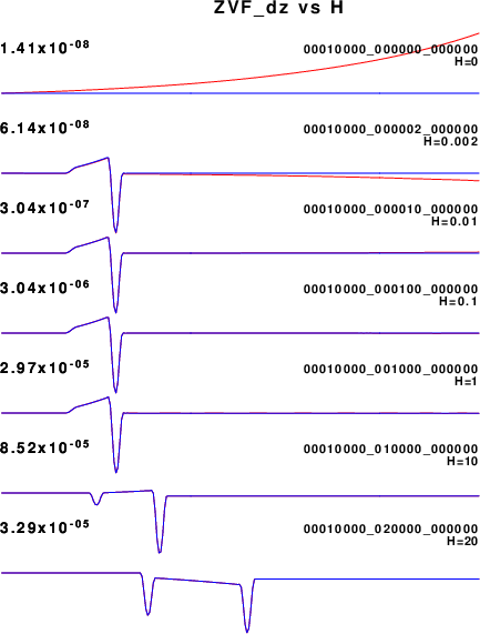
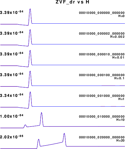
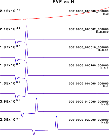
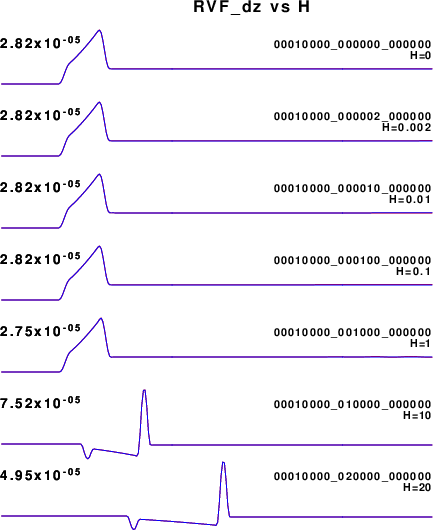
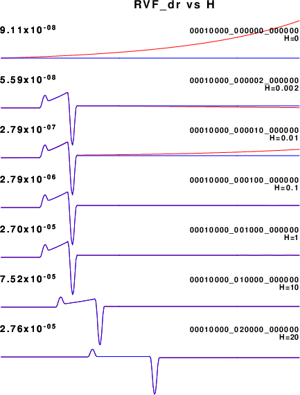
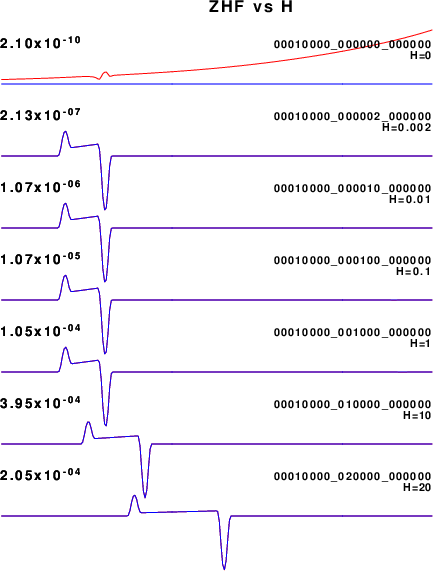
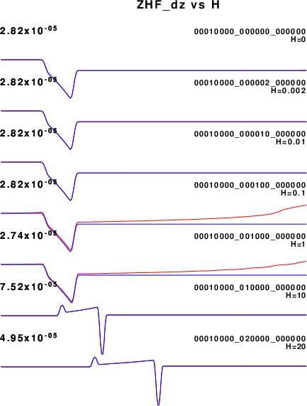
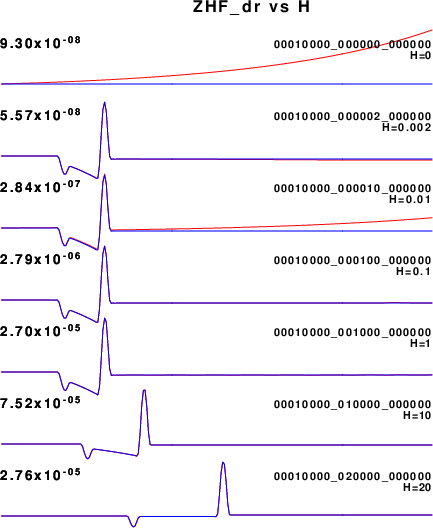
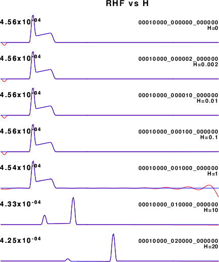
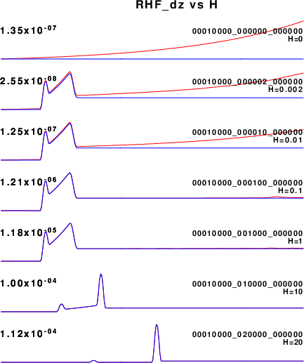
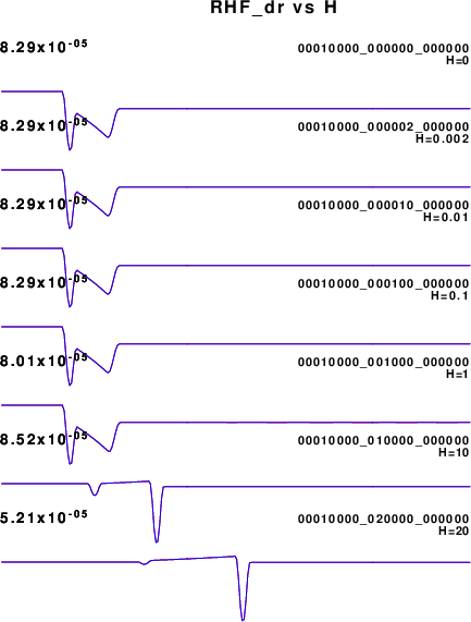
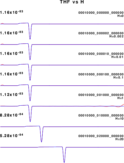
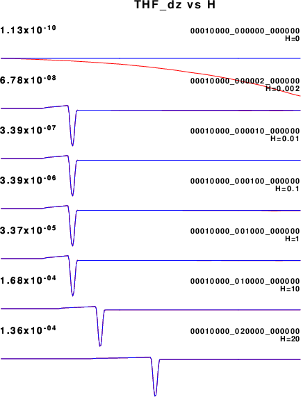
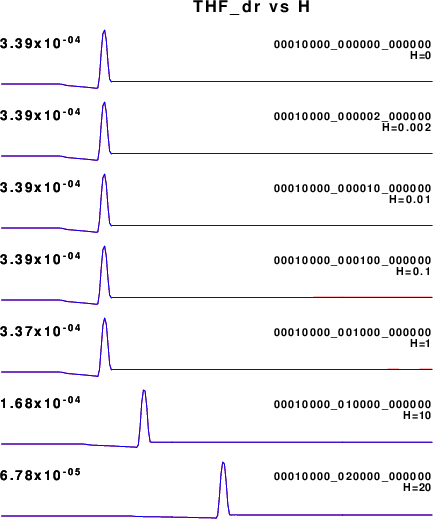
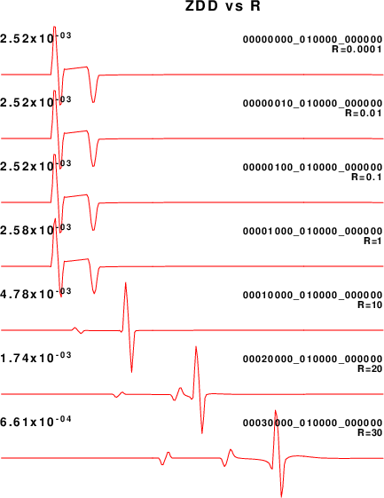
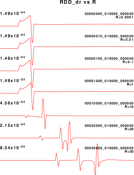
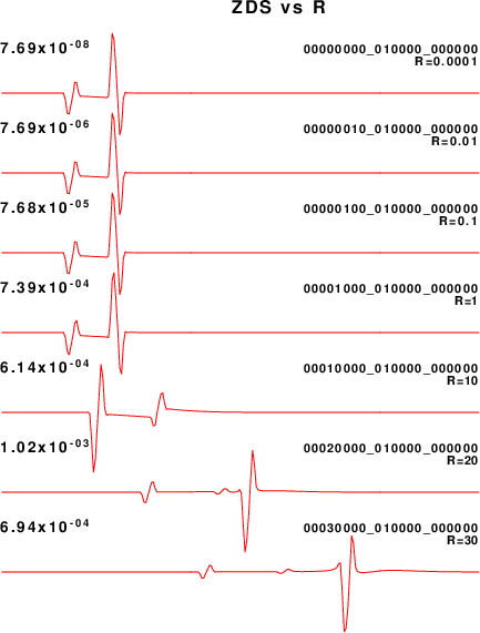
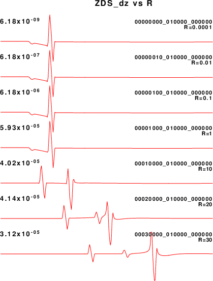
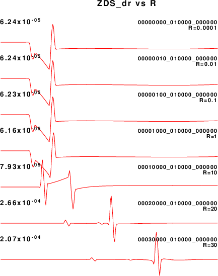
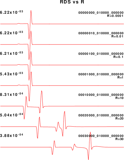
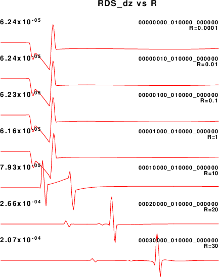
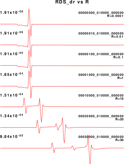
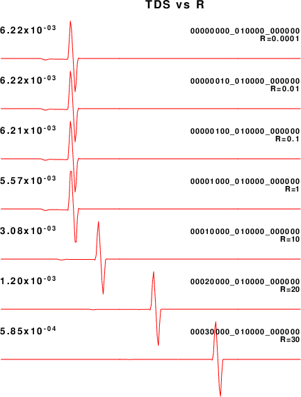
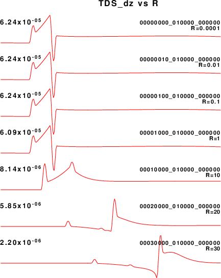
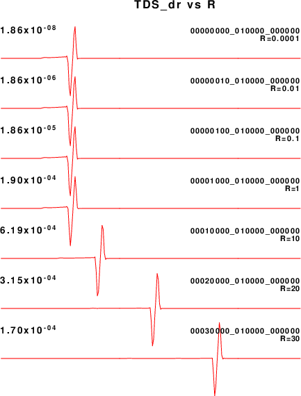
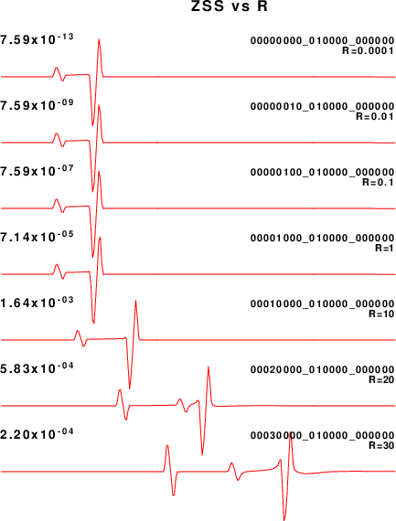
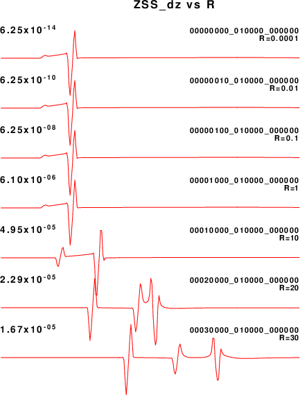
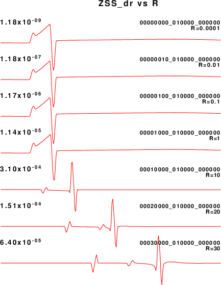
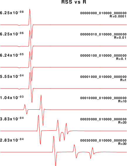
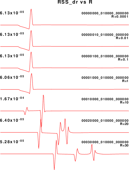
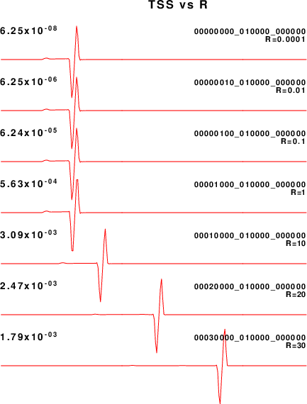
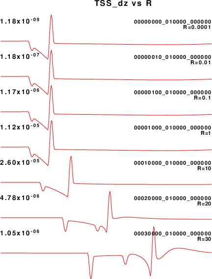
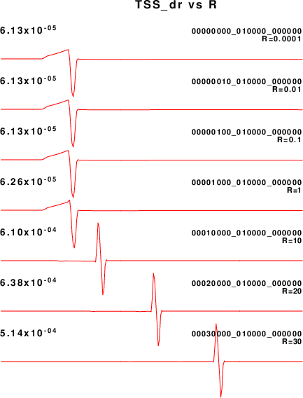
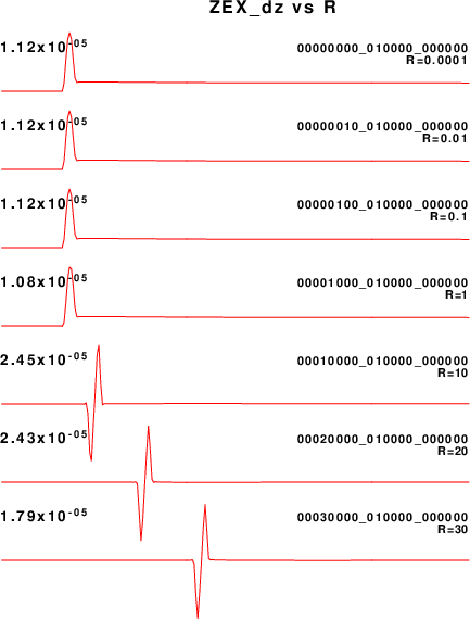
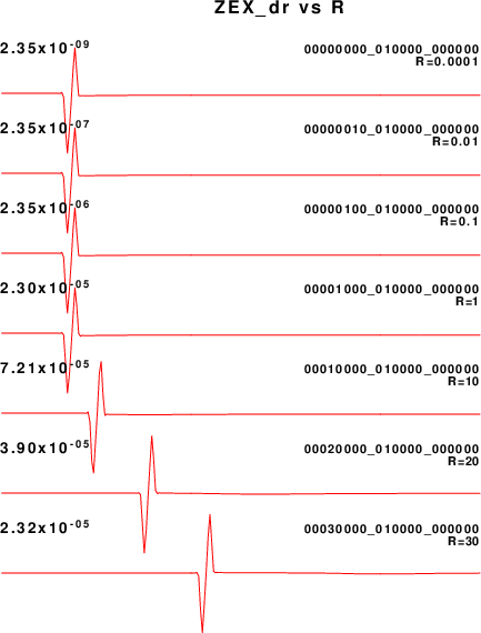
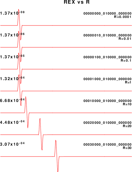
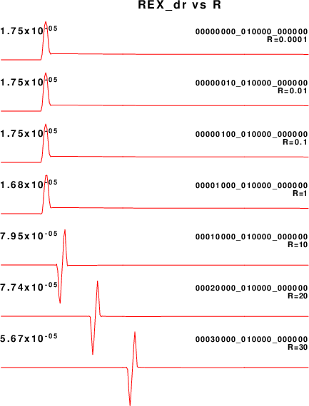
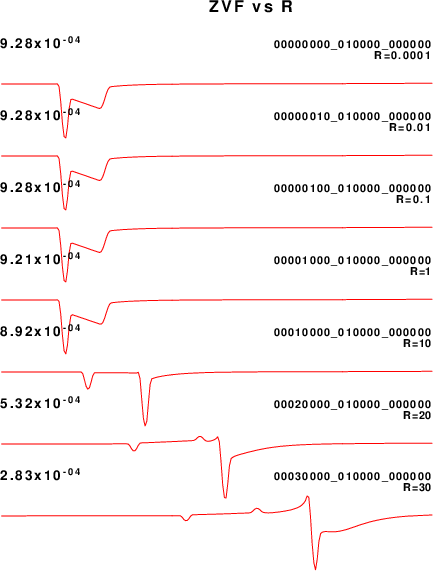
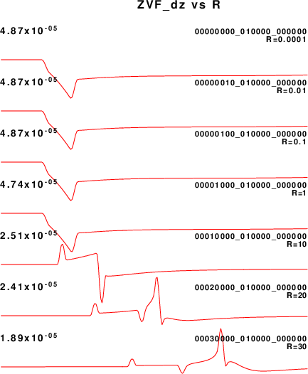
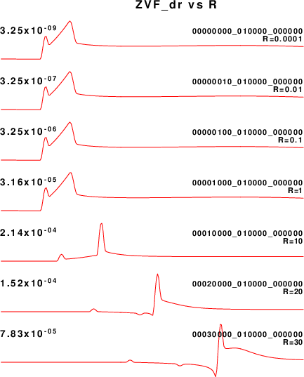
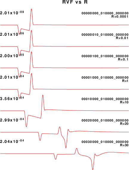
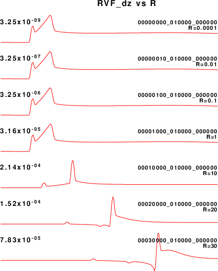
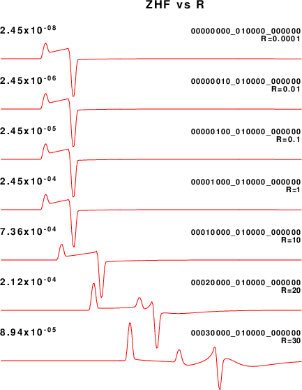
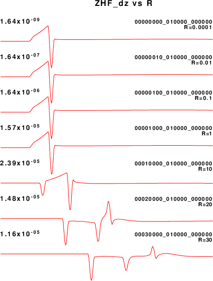
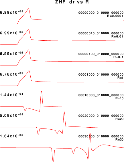
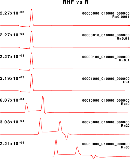
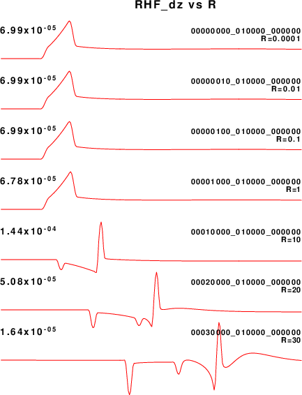
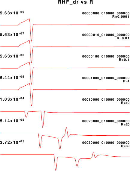
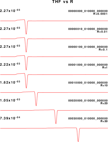
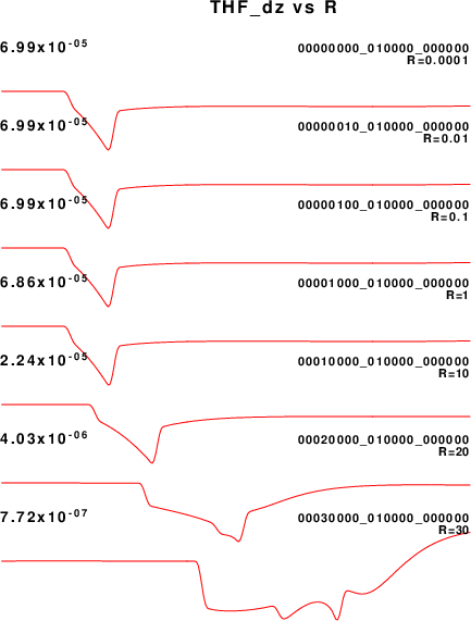
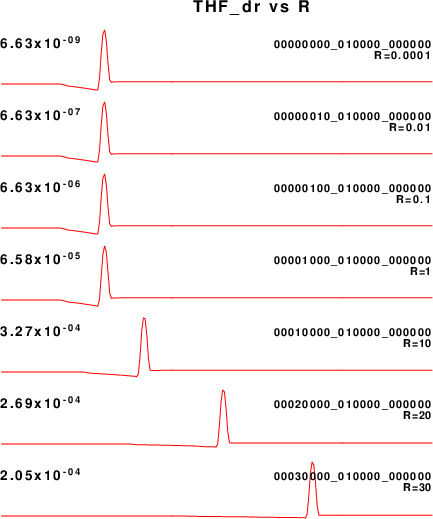
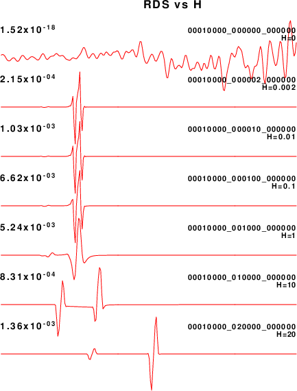
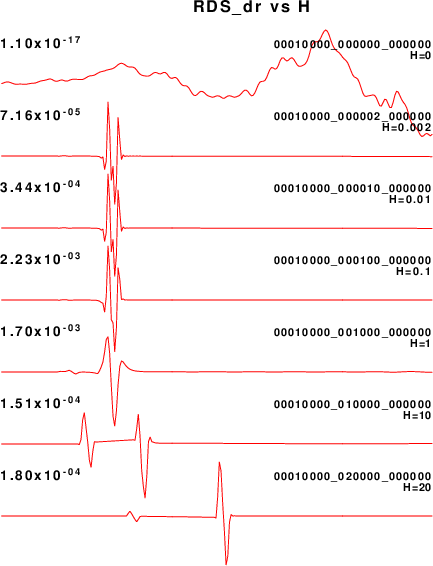
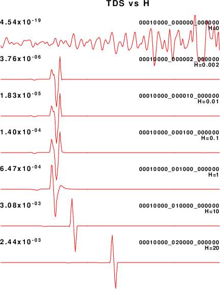
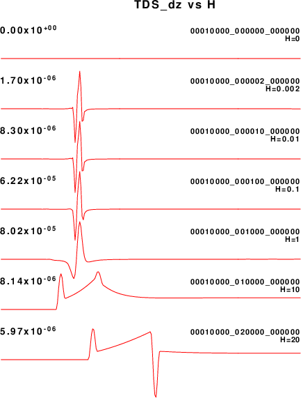
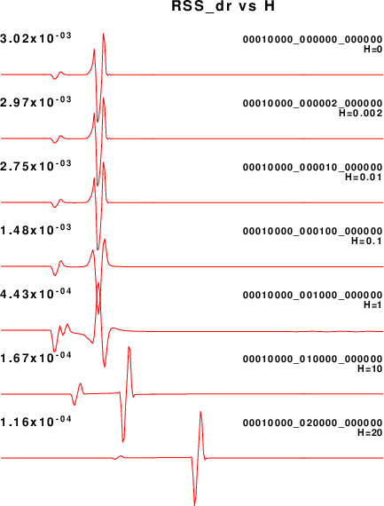
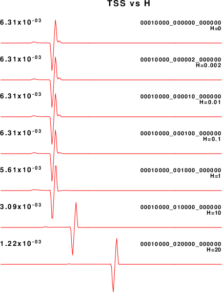
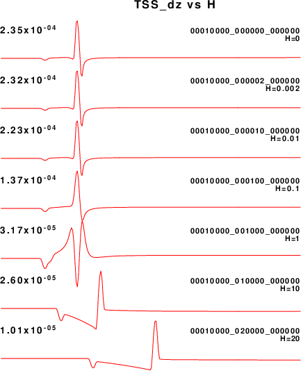
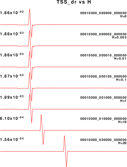
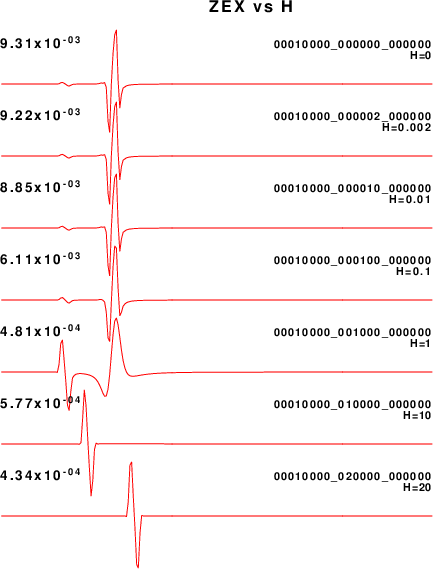
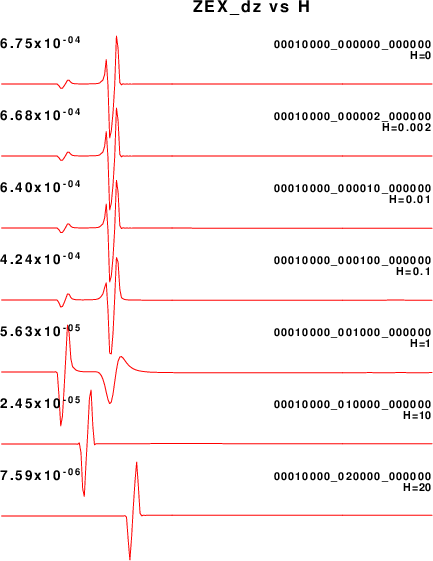
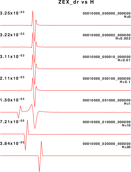
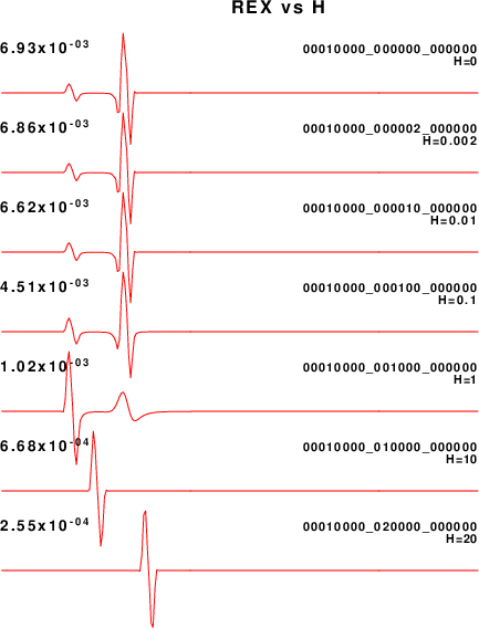
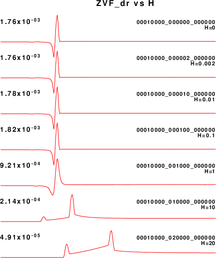
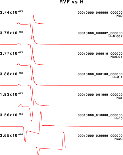
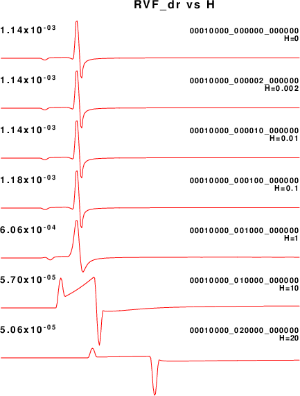
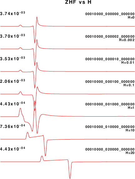
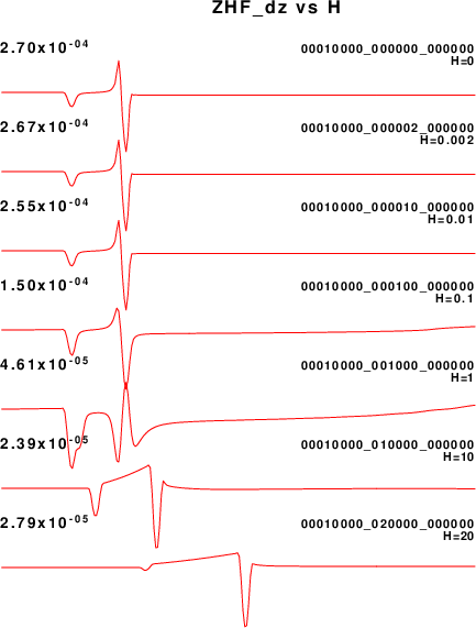
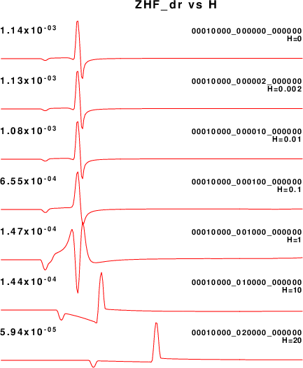
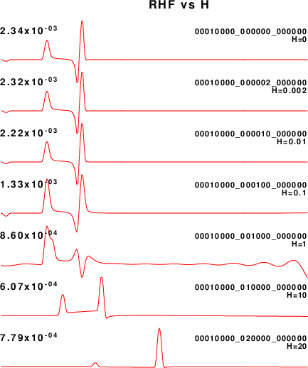
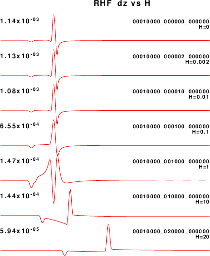
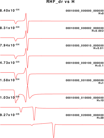
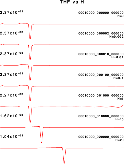
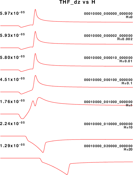
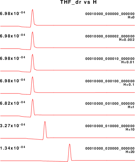
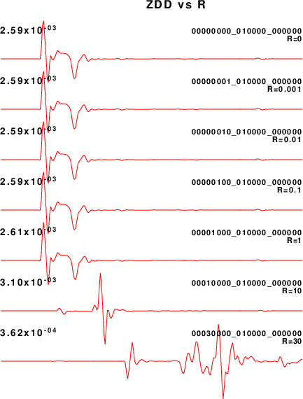
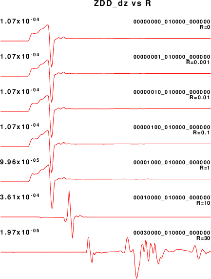
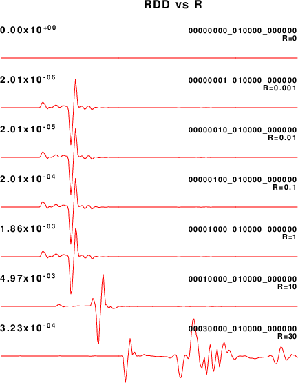
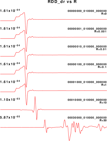
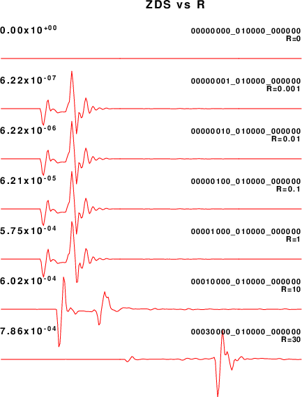
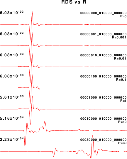
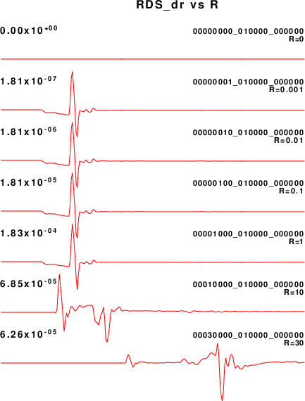
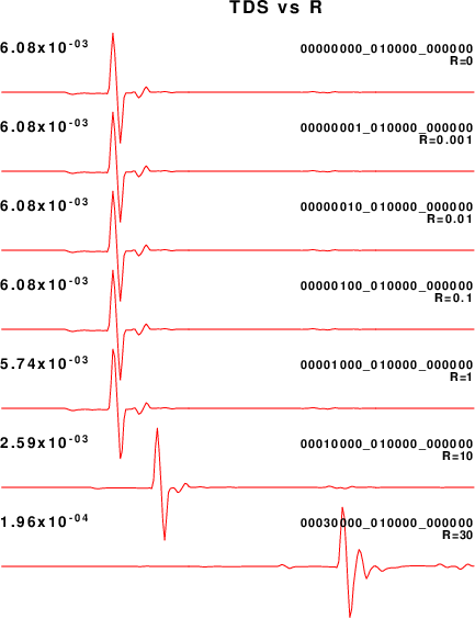
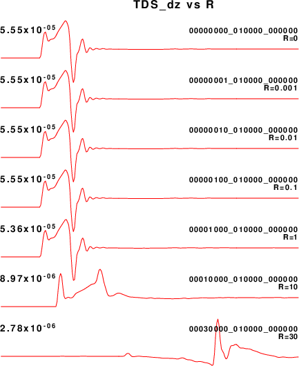
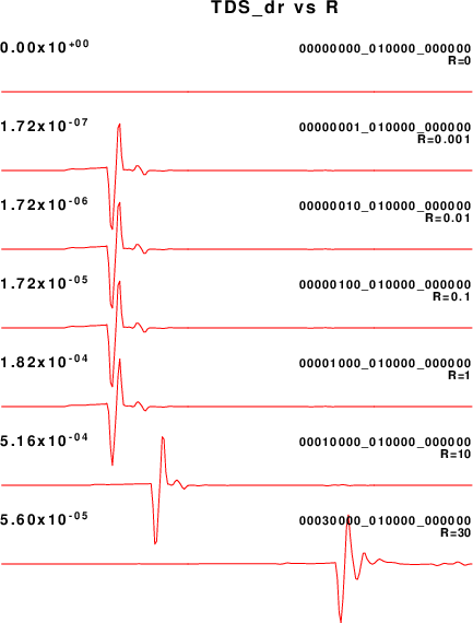
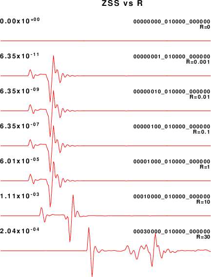
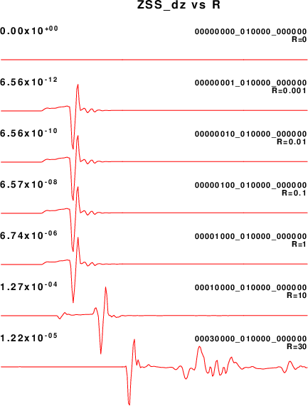
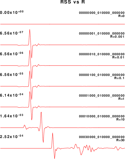
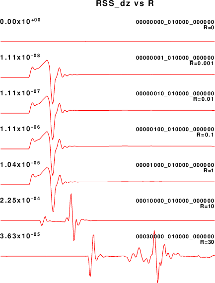
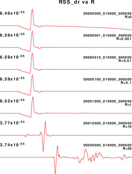
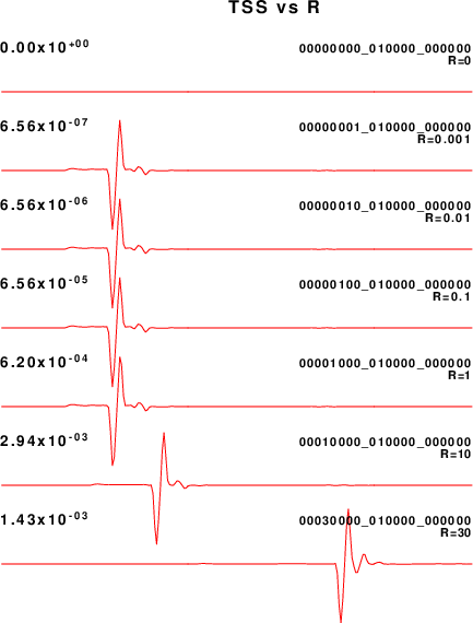
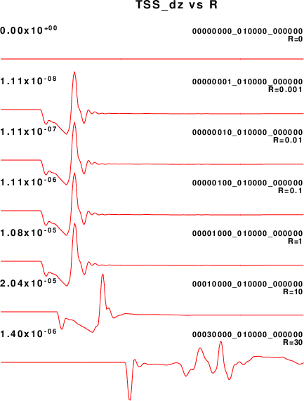
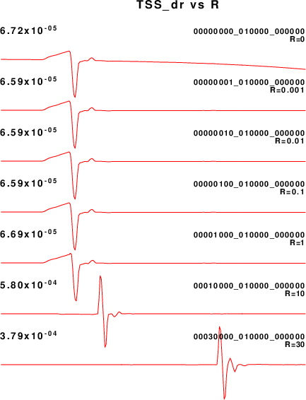
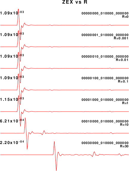
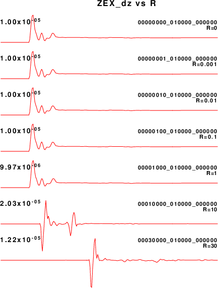
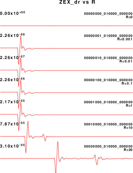
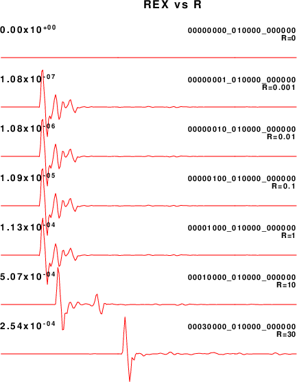
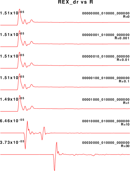
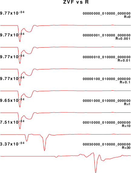
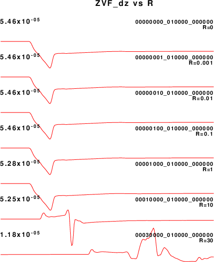
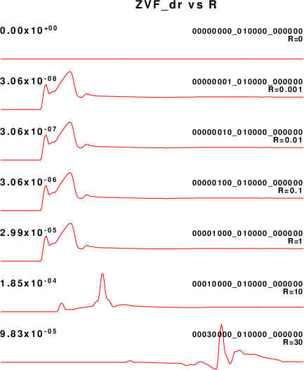
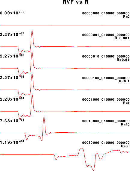
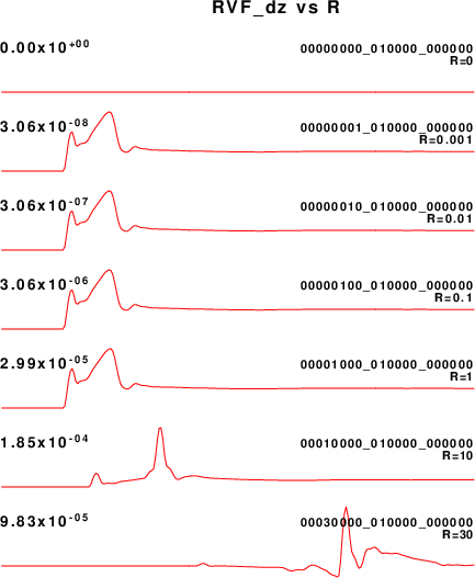
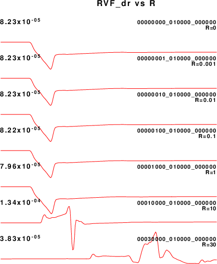
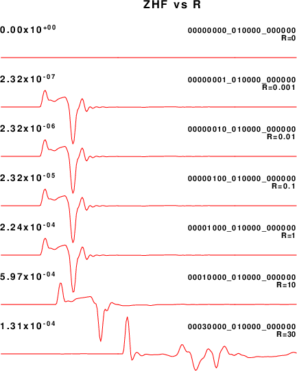
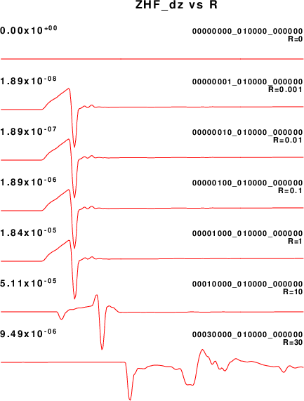
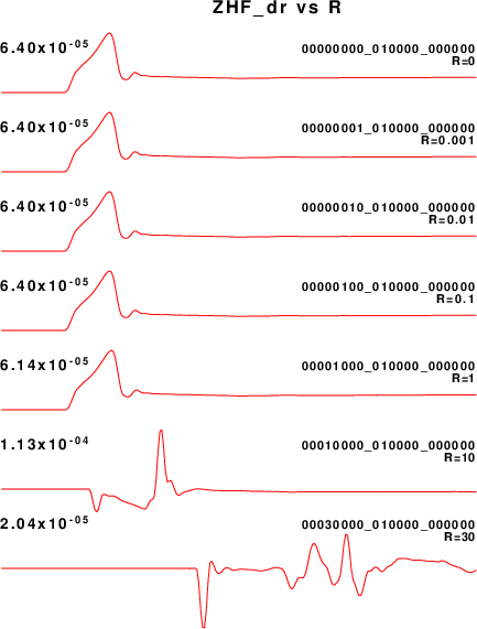
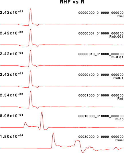
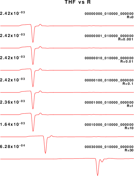
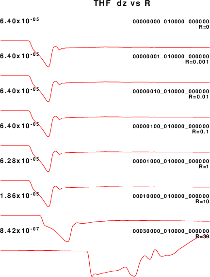
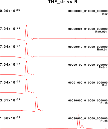
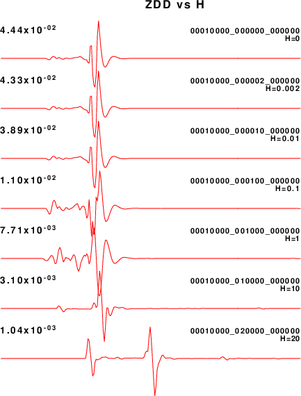
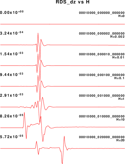
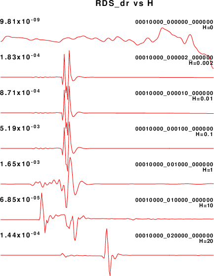
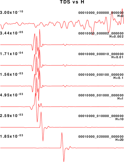
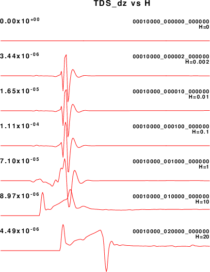
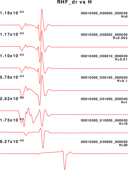
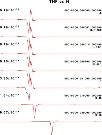
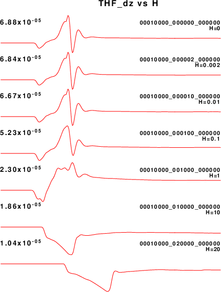
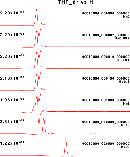
The results of the comparison are displayed in figures seen by clicking on the links of the next table. In these figures, the red curve is the true solution from hwhole96strain and the blue curve is from hspec96strain. Each comparison is annotated with the peak amplitude, the leading part of the file name which indicates distance, source and receiver depths, and the radial distance, as R=0.0001km, for example.

In general the comparison is very good. It is only when R=0.0001 km for H=10.0 km that there are problems. The SS amplitudes are very small and the waveform is noisy. This is expected. For the SS source and a near vertical ray, the P, SV and SH amplitudes are nodal. In this case the noise is acceptable.

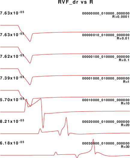
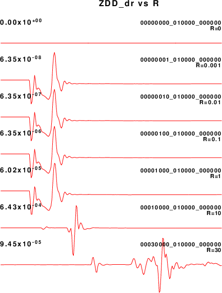
More problematic are the d /dr partial derivatives of RDS, TDS and TSS, which have large amplitudes and in some case an exponential increase in the signal with time.

The d /dz partial derivative of RHF has some low frequency problems at R=30 km, but the amplitude of the partial decreases with distance.

Thus the Green's functions and partial derivatives seem OK for 0.00001 < (R/H) < 3 .

Variation of epicentral distance for H=10km Variation of source depth for R=10km

Green's function d /dz d /dr

ZDD d ZDD/dz d ZDD/dr

RDD d RDD/dz d RDD/dr

ZDS d ZDS/dz d ZDS/dr

RDS d RDS/dz d RDS/dr

TDS d TDS/dz d TDS/dr

ZSS d ZSS/dz d ZSS/dr

RSS d RSS/dz d RSS/dr

TSS d TSS/dz d TSS/dr

ZEX d ZEX/dz d ZEX/dr

REX d REX/dz d REX/dr

ZVF d ZVF/dz d ZVF/dr

RVF d RVF/dz d RVF/dr

ZHF d ZHF/dz d ZHF/dr

RHF d RHF/dz d RHF/dr

THF d THF/dz d THF/dr

Green's function d /dz d /dr

ZDD d ZDD/dz d ZDD/dr

RDD d RDD/dz d RDD/dr

ZDS d ZDS/dz d ZDS/dr

RDS d RDS/dz d RDS/dr

TDS d TDS/dz d TDS/dr

ZSS d ZSS/dz d ZSS/dr

RSS d RSS/dz d RSS/dr

TSS d TSS/dz d TSS/dr

ZEX d ZEX/dz d ZEX/dr

REX d REX/dz d REX/dr

ZVF d ZVF/dz d ZVF/dr

RVF d RVF/dz d RVF/dr

ZHF d ZHF/dz d ZHF/dr

RHF d RHF/dz d RHF/dr

THF d THF/dz d THF/dr

Discussion

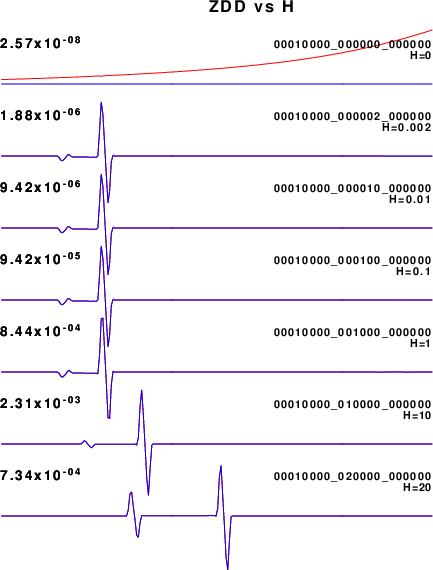
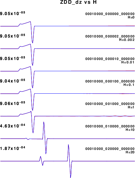
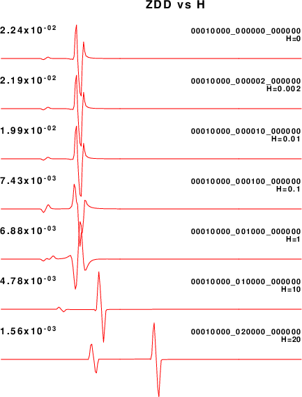
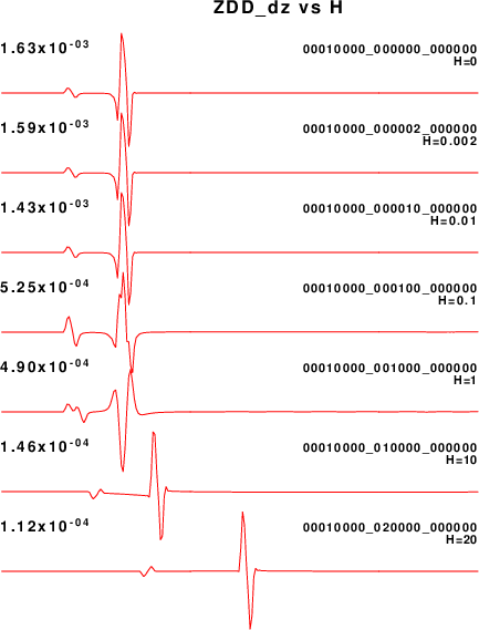
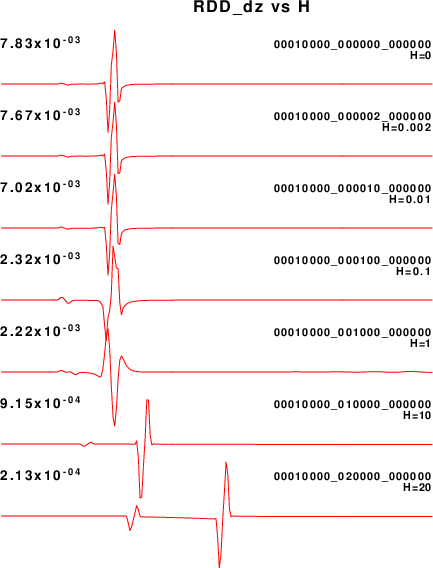
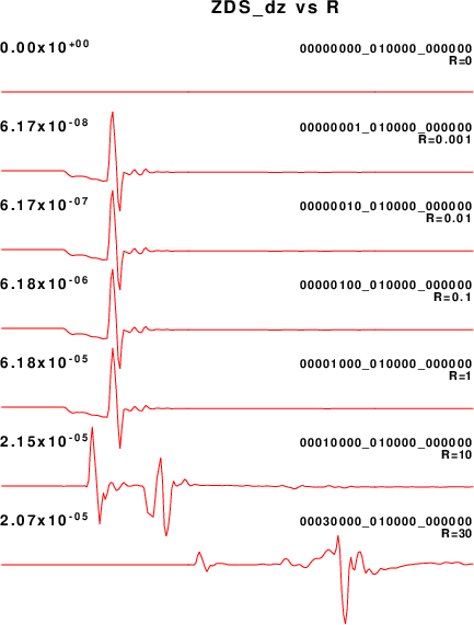
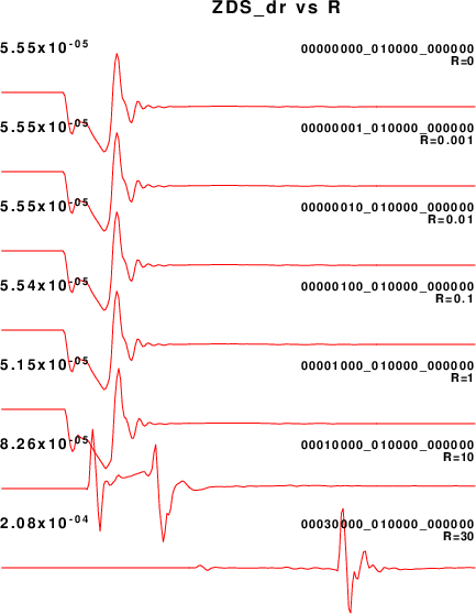
The comparison between the results from hwhole96strain and hspec96strain are very good the fixed source depth and variable epicentral distance, because of the care taken in coding the Bessel functions and their radial derivatives for small epicentral distances.

However there are problems as the vertical separation becomes small. This is seen in the d/dr derivatives of RDS, ZDD and ZED, and the d/dz derivatives of RDD, REX, RHF, RSS and ZDS. When the vertical separation between the source and receiver is small, then the ray is horizontal and the expected amplitudes of many of the Green's functions is zero. Thus the low frequency trend may reflect numerical error as much as the breakdown of the algorithm,

Thus more work has to be done when H is small compared to R.

Halfspace Test

This set of tests considers both a uniform halfspace model HALF.mod and a layered halfspace model CUS.mod.

Uniform halfspace

The halfspace velocity model, named HALF.mod is created with this shell script:


cat > HALF.mod << EOF
MODEL.01
Simple wholespace model
ISOTROPIC
KGS
FLAT EARTH
1-D
CONSTANT VELOCITY
LINE08
LINE09
LINE10
LINE11
H(KM) VP(KM/S) VS(KM/S) RHO(GM/CC) QP QS ETAP ETAS FREFP FREFS
40.0  6.00       3.5     2.7        0  0  0    0     1     1
EOF

The synthetics are made using the following script which is invoked with the source depth and epicentral distance on the command line. This script differs from the one above in the model used but more importantly in the hprep96 flag -TF which causes the model to be considered as a halfspace with a free surface.

#!/bin/sh H=$1 R=$2 cat > dfile << EOF ${R} 0.05 256 0 0 EOF hprep96 -M HALF.mod -d dfile -HS ${H} -HR 0 -TF -BH hwhole96strain hpulse96strain -TEST1 -V -p -l 2 -FMT 2

Layered Halfspace

The the layered halfspace velocity model, named CUS.mod is created with this shell script:


cat > CUS.mod << EOF
MODEL.01
CUS Model with Q from simple gamma values
ISOTROPIC
KGS
FLAT EARTH
1-D
CONSTANT VELOCITY
LINE08
LINE09
LINE10
LINE11
  H(KM) VP(KM/S) VS(KM/S) RHO(GM/CC)   QP   QS  ETAP  ETAS  FREFP  FREFS
  1.0000  5.0000  2.8900  2.5000 0.172E-02 0.387E-02 0.00  0.00  1.00  1.00 
  9.0000  6.1000  3.5200  2.7300 0.160E-02 0.363E-02 0.00  0.00  1.00  1.00 
 10.0000  6.4000  3.7000  2.8200 0.149E-02 0.336E-02 0.00  0.00  1.00  1.00 
 20.0000  6.7000  3.8700  2.9020 0.000E-04 0.000E-04 0.00  0.00  1.00  1.00 
  0.0000  8.1500  4.7000  3.3640 0.194E-02 0.431E-02 0.00  0.00  1.00  1.00 
EOF

#!/bin/sh H=$1 R=$2 cat > dfile << EOF ${R} 0.05 256 0 0 EOF hprep96 -M CUS.mod -d dfile -HS ${H} -HR 0 -TF -BH hwhole96strain hpulse96strain -TEST1 -V -p -l 2 -FMT 2

Discussion

The computations look good.

3. Summary

This tutorial shows how to evaluate imperfections in the computations. It is obvious that there will be some problems in computing strain synthetics as the vertical positions source and receiver become closer.